
The setup of the double slit experiment
“I think I can safely say that nobody understands quantum mechanics.” , Richard Feynman, 1965
“The only difference between a probabilistic classical world and the equations of the quantum world is that somehow or other it appears as if the probabilities would have to go negative”, Richard Feynman, 1982
For much of the history of mankind, people believed that the ultimate “theory of everything” would be of the “billiard ball” type. That is, at the end of the day, everything is composed of some elementary particles and adjacent particles interact with one another according to some well specified laws. The types of particles and laws might differ, but not the general shape of the theory. Note that this in particular means that a system of \(N\) particles can be simulated by a computer with \(poly(N)\) memory and time.
Alas, in the beginning of the 20th century, several experimental results were calling into question the “billiard ball” theory of the world. One such experiment is the famous “double slit” experiment. Suppose we shoot an electron at a wall that has a single slit at position \(i\) and put somewhere behind this slit a detector. If we let \(p_i\) be the probability that the electron goes through the slit and let \(q_i\) be the probability that conditioned on this event, the electron hits this detector, then the fraction of times the electron hits our detector should be (and indeed is) \(\alpha = p_iq_i\). Similarly, if we close this slit and open a second slit at position \(j\) then the new fraction of times the electron hits our detector will be \(\beta=p_jq_j\). Now if we open both slits then it seems that the fraction should be \(\alpha+\beta\) and in particular, “obviously” the probability that the electron hits our detector should only increase if we open a second slit. However, this is not what actually happens when we run this experiment. It can be that the detector is hit a smaller number of times when two slits are open than when only a single one hits. It’s almost as if the electron checks whether two slits are open, and if they are, it changes the path it takes. If we try to “catch the electron in the act” and place a detector right next to each slit so we can count which electron went through which slit then something even more bizzare happened. The mere fact that we measured the electron path changes the actual path it takes, and now this “destructive interference” pattern is gone and the detector will be hit \(\alpha+\beta\) fraction of the time.
The setup of the double slit experiment
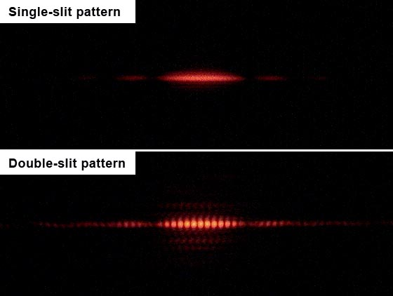
In the double slit experiment, opening two slits can actually cause some positions to receive fewer electrons than before.
Quantum mechanics is a mathematical theory that allows us to calculate and predict the results of this and many other examples. If you think of quantum as an explanation as to what “really” goes on in the world, it can be rather confusing. However, if you simply “shut up and calculate” then it works amazingly well at predicting the results of a great many experiments.
In the double slit experiment, quantum mechanics still allows to compute numbers \(\alpha\) and \(\beta\) that denote “probabilities” that the first and second electrons hit the detector. The only difference that in quantum mechanics these probabilities might be negative numbers. However, probabilities can only be negative when no one is looking at them. When we actually measure what happened to the detector, we make the probabilities positive by squaring them. So, if only the first slit is open, the detector will be hit \(\alpha^2\) fraction of the time. If only the second slit is open, the detector will be hit \(\beta^2\) fraction of the time. And if both slits are open, the detector will be hit \((\alpha+\beta)^2\) fraction of the time. Note that it can well be that \((\alpha+\beta)^2 < \alpha^2 + \beta^2\) and so this calculation explains why the number of times a detector is hit when two slits are open might be smaller than the number of times it is hit when either slit is open. If you haven’t seen it before, it may seem like complete nonsense and at this point I’ll have to politely point you back to the part where I said we should not question quantum mechanics but simply “shut up and calculate”.1
Some of the counterintuitive properties that arise from these negative probabilities include:
Again, as counter-intuitive as these concepts are, they have been experimentally confirmed, so we just have to live with them.
One of the strange aspects of the quantum-mechanical picture of the world is that unlike in the billiard ball example, there is no obvious algorithm to simulate the evolution of \(n\) particles over \(t\) time periods in \(poly(n,t)\) steps. In fact, the natural way to simulate \(n\) quantum particles will require a number of steps that is exponential in \(n\). This is a huge headache for scientists that actually need to do these calculations in practice.
In the 1981, physicist Richard Feynman proposed to “turn this lemon to lemonade” by making the following almost tautological observation:
If a physical system cannot be simulated by a computer in \(T\) steps, the system can be considered as performing a computation that would take more than \(T\) steps
So, he asked whether one could design a quantum system such that its outcome \(y\) based on the initial condition \(x\) would be some function \(y=f(x)\) such that (a) we don’t know how to efficiently compute in any other way, and (b) is actually useful for something.2 In 1985, David Deutsch formally suggested the notion of a quantum Turing machine, and the model has been since refined in works of Detusch and Josza and Bernstein and Vazirani. Such a system is now known as a quantum computer.
For a while these hypothetical quantum computers seemed useful for one of two things. First, to provide a general-purpose mechanism to simulate a variety of the real quantum systems that people care about. Second, as a challenge to the theory of computation’s approach to model efficient computation by Turing machines, though a challenge that has little bearing to practice, given that this theoretical “extra power” of quantum computer seemed to offer little advantage in the problems people actually want to solve such as combinatorial optimization, machine learning, data structures, etc..
To a significant extent, this is still true today. We have no real evidence that quantum computers, if built, will offer truly significant3 advantage in 99% of the applications of computing.4 However, there is one cryptography-sized exception: In 1994 Peter Shor showed that quantum computers can solve the integer factoring and discrete logarithm in polynomial time. This result has captured the imagination of a great many people, and completely energized research into quantum computing.
This is both because the hardness of these particular problems provides the foundations for securing such a huge part of our communications (and these days, our economy), as well as it was a powerful demonstration that quantum computers could turn out to be useful for problems that a-priori seemd to have nothing to do with quantum physics. As we’ll discuss later, at the moment there are several intensive efforts to construct large scale quantum computers. It seems safe to say that, as far as we know, in the next five years or so there will not be a quantum computer large enough to factor, say, a \(1024\) bit number, but there it is quite possible that some quantum computer will be built that is strong enough to achieve some task that is too inefficient to achieve with a non-quantum or “classical” computer (or at least requires more resources classically than it would for this computer). When and if such a computer is built that can break reasonable parameters of Diffie Hellman, RSA and elliptic curve cryptography is anybody’s guess. It could also be a “self destroying prophecy” whereby the existence of a small-scale quantum computer would cause everyone to shift away to lattice-based crypto which in turn will diminish the motivation to invest the huge resources needed to build a large scale quantum computer.5
The above summary might be all that you need to know as a cryptographer, and enough motivation to study lattice-based cryptography as we do in this course. However, because quantum computing is such a beautiful and (like cryptography) counter-intuitive concept, we will try to give at least a hint of what is it about and how does Shor’s algorithm work.
We now present some of the basic notions in quantum information. It is very useful to contrast these notions to the setting of probabilistic systems and see how “negative probabilities” make a difference. This discussion is somewhat brief. The chapter on quantum computation in my book with Arora (see draft here) is one relatively short resource that contains essentially everything we discuss here. See also this blog post of Aaronson for a high level explanation of Shor’s algorithm which ends with links to several more detailed expositions. See also this lecture of Aaronson for a great discussion of the feasibility of quantum computing (Aaronson’s course lecture notes and the book that they spawned are fantastic reads as well).
States: We will consider a simple quantum system that includes \(n\) objects (e.g., electrons/photons/transistors/etc..) each of which can be in either an “on” or “off” state - i.e., each of them can encode a single bit of information, but to emphasize the “quantumness” we will call it a qubit. A probability distribution over such a system can be described as a \(2^n\) dimensional vector \(v\) with non-negative entries summing up to \(1\), where for every \(x\in{\{0,1\}}^n\), \(v_x\) denotes the probability that the system is in state \(x\). As we mentioned, quantum mechanics allows negative (in fact even complex) probabilities and so a quantum state of the system can be described as a \(2^n\) dimensional vector \(v\) such that \(\|v\|^2 = \sum_x |v_x|^2 = 1\).
Measurement: Suppose that we were in the classical probabilistic setting, and that the \(n\) bits are simply random coins. Thus we can describe the state of the system by the \(2^n\)-dimensional vector \(v\) such that \(v_x=2^{-n}\) for all \(x\). If we measure the system and see what the coins came out, we will get the value \(x\) with probability \(v_x\). Naturally, if we measure the system twice we will get the same result. Thus, after we see that the coin is \(x\), the new state of the system collapses to a vector \(v\) such that \(v_y = 1\) if \(y=x\) and \(v_y=0\) if \(y\neq x\). In a quantum state, we do the same thing: if we measure a vector \(v\) corresponds to turning it with probability \(|v_x|^2\) into a vector that has \(1\) on coordinate \(x\) and zero on all the other coordinates.
Operations: In the classical probabilistic setting, if we have a system in state \(v\) and we apply some function \(f:{\{0,1\}}^n\rightarrow{\{0,1\}}^n\) then this transforms \(v\) to the state \(w\) such that \(w_y = \sum_{x:f(x)=y} v_x\).
Another way to state this, is that \(w=M_f\) where \(M_f\) is the matrix such that \(M_{f(x),x}=1\) for all \(x\) and all other entries are \(0\). If we toss a coin and decide with probability \(1/2\) to apply \(f\) and with probability \(1/2\) to apply \(g\), this corresponds to the matrix \((1/2)M_f + (1/2)M_g\). More generally, the set of operations that we can apply can be captured as the set of convex combinations of all such matrices- this is simply the set of non-negative matrices whose columns all sum up to \(1\)- the stochastic matrices. In the quantum case, the operations we can apply to a quantum state are encoded as a unitary matrix, which is a matrix \(M\) such that \(\|Mv\|=\|v\|\) for all vectors \(v\).
Elementary operations: Of course, even in the probabilistic setting, not every function \(f:{\{0,1\}}^n\rightarrow{\{0,1\}}^n\) is efficiently computable. We think of a function as efficiently computable if it is composed of polynomially many elementary operations, that involve at most \(2\) or \(3\) bits or so (i.e., Boolean gates). That is, we say that a matrix \(M\) is elementary if it only modifies three bits. That is, \(M\) is obtained by “lifting” some \(8\times 8\) matrix \(M'\) that operates on three bits \(i,j,k\), leaving all the rest of the bits intact. Formally, given an \(8\times 8\) matrix \(M'\) (indexed by strings in \({\{0,1\}}^3\)) and three distinct indices \(i<j<k \in \{1,\ldots,n\}\) we define the \(n\)-lift of \(M'\) with indices \(i,j,k\) to be the \(2^n\times 2^n\) matrix \(M\) such that for every strings \(x\) and \(y\) that agree with each other on all coordinates except possibly \(i,j,k\), \(M_{x,y}=M'_{x_ix_jx_k,y_iy_jy_k}\) and otherwise \(M_{x,y}=0\). Note that if \(M'\) is of the form \(M'_f\) for some function \(f:{\{0,1\}}^3\rightarrow{\{0,1\}}^3\) then \(M=M_g\) where \(g:{\{0,1\}}^n\rightarrow{\{0,1\}}^n\) is defined as \(g(x)=f(x_ix_jx_k)\). We define \(M\) as an elementary stochastic matrix or a probabilistic gate if \(M\) is equal to an \(n\) lift of some stochastic \(8\times 8\) matrix \(M'\). The quantum case is similar: a quantum gate is a \(2^n\times 2^n\) matrix that is an \(N\) lift of some unitary \(8\times 8\) matrix \(M'\). It is an exercise to prove that lifting preserves stochasticity and unitarity. That is, every probabilistic gate is a stochastic matrix and every quantum gate is a unitary matrix.
Complexity: For every stochastic matrix \(M\) we can define its randomized complexity, denoted as \(R(M)\) to be the minimum number \(T\) such that \(M\) is can be (approximately) obtained by combining \(T\) elemntary probabilistic gates. To be concrete, we can define \(R(M)\) to be the minimum \(T\) such that there exists \(T\) elementary matrices \(M_1,\ldots,M_T\) such that for every \(x\), \(\sum_y |M_{y,x}-(M_T\cdots M_1)_{y,x}|<0.1\). (It can be shown that \(R(M)\) is finite and in fact at most \(10^n\) for every \(M\); we can do so by writing \(M\) as a convex combination of function and writing every function as a composition of functions that map a single string \(x\) to \(y\), keeping all other inputs intact.) We will say that a probabilistic process \(M\) mapping distributions on \({\{0,1\}}^n\) to distributions on \({\{0,1\}}^n\) is efficiently classically computable if \(R(M) \leq poly(n)\). If \(M\) is a unitary matrix, then we define the quantum complexity of \(M\), denoted as \(Q(M)\), to be the minimum number \(T\) such that there are quantum gates \(M_1,\ldots,M_T\) satisfying that for every \(x\), \(\sum_y |M_{y,x}-(M_T \cdots M_1)_{y,x}|^2 < 0.1\).
We say that \(M\) is efficiently quantumly computable if \(Q(M)\leq poly(n)\).
Computing functions: We have defined what it means for an operator to be probabilistically or quantumly efficiently computable, but we typically are interested in computing some function \(f:{\{0,1\}}^m\rightarrow{\{0,1\}}^\ell\). The idea is that we say that \(f\) is efficiently computable if the corresponding operator is efficiently computable, except that we also allow to use extra memory and so to embed \(f\) in some \(n=poly(m)\). We define \(f\) to be efficiently classically computable if there is some \(n=poly(m)\) such that the operator \(M_g\) is efficiently classically computable where \(g:{\{0,1\}}^n\rightarrow{\{0,1\}}^n\) is defined such that \(g(x_1,\ldots,x_n)=f(x_1,\ldots,x_m)\). In the quantum case we have a slight twist since the operator \(M_g\) is not necessarily a unitary matrix.6 Therefore we say that \(f\) is efficiently quantumly computable if there is \(n=poly(m)\) such that the operator \(M_q\) is efficiently quantumly computable where \(g:{\{0,1\}}^n\rightarrow{\{0,1\}}^n\) is defined as \(g(x_1,\ldots,x_n) = x_1\cdots x_m \|( f(x_1\cdots x_m)0^{n-m-\ell}\; \oplus \; x_{m+1}\cdots x_n)\).
Quantum and classical computation: The way we defined what it means for a function to be efficiently quantumly computable, it might not be clear that if \(f:{\{0,1\}}^m\rightarrow{\{0,1\}}^\ell\) is a function that we can compute by a polynomial size Boolean circuit (e.g., combining polynomially many AND, OR and NOT gates) then it is also quantumly efficiently computable. The idea is that for every gate \(g:{\{0,1\}}^2\rightarrow{\{0,1\}}\) we can define an \(8\times 8\) unitary matrix \(M_h\) where \(h:{\{0,1\}}^3\rightarrow{\{0,1\}}^3\) have the form \(h(a,b,c)=a,b,c\oplus g(a,b)\). So, if \(f\) has a circuit of \(s\) gates, then we can dedicate an extra bit for every one of these gates and then run the corresponding \(s\) unitary operations one by one, at the end of which we will get an operator that computes the mapping \(x_1,\ldots,x_{m+\ell+s} = x_1\cdots x_m \| x_{m+1}\cdots x_{m+s} \oplus f(x_1,\ldots,x_m)\|g(x_1\ldots x_m)\) where the the \(\ell+i^{th}\) bit of \(g(x_1,\ldots,x_n)\) is the result of applying the \(i^{th}\) gate in the calculation of \(f(x_1,\ldots,x_m)\). So this is “almost” what we wanted except that we have this “extra junk” that we need to get rid of. The idea is that we now simply run the same computation again which will basically we mean we XOR another copy of \(g(x_1,\ldots,x_m)\) to the last \(s\) bits, but since \(g(x)\oplus g(x) = 0^s\) we get that we compute the map \(x \mapsto x_1\cdots x_m \| (f(x_1,\ldots,x_m)0^s \;\oplus\; x_{m+1}\cdots x_{m+\ell+s})\) as desired.
The “obviously exponential” fallacy: A priori it might seem “obvious” that quantum computing is exponentially powerful, since to compute a quantum computation on \(n\) bits we need to maintain the \(2^n\) dimensional state vector and apply \(2^n\times 2^n\) matrices to it. Indeed popular descriptions of quantum computing (too) often say something along the lines that the difference between quantum and classical computer is that a classic bit can either be zero or one while a qubit can be in both states at once, and so in many qubits a quantum computer can perform exponentially many computations at once. Depending on how you interpret this, this description is either false or would apply equally well to probabilistic computation. However, for probabilistic computation it is a not too hard exercise to show that if \(f:{\{0,1\}}^m\rightarrow{\{0,1\}}^n\) is an efficiently computable function then it has a polynomial size circuit of AND, OR and NOT gates.7 Moreover, this “obvious” approach for simulating a quantum computation will take not just exponential time but exponential space as well, while it is not hard to show that using a simple recursive formula one can calculate the final quantum state using polynomial space (in physics parlance this is known as “Feynman path integrals”). So, the exponentially long vector description by itself does not imply that quantum computers are exponentially powerful. Indeed, we cannot prove that they are (since in particular we can’t prove that every polynomial space calculation can be done in polynomial time, in complexity parlance we don’t know how to rule out that \(P=PSPACE\)), but we do have some problems (integer factoring most prominently) for which they do provide exponential speedup over the currently best known classical (deterministic or probabilistic) algorithms.
To realize quantum computation one needs to create a system with \(n\) independent binary states (i.e., “qubits”), and be able to manipulate small subsets of two or three of these qubits to change their state. While by the way we defined operations above it might seem that one needs to be able to perform arbitrary unitary operations on these two or three qubits, it turns out that there several choices for universal sets - a small constant number of gates that generate all others. The biggest challenge is how to keep the system from being measured and collapsing to a single classical combination of states. This is sometimes known as the coherence time of the system. The threshold theorem says that there is some absolute constant level of errors \(\tau\) so that if errors are created at every gate at rate smaller than \(\tau\) then we can recover from those and perform arbitrary long computations. (Of course there are different ways to model the errors and so there are actually several threshold theorems corresponding to various noise models).
There have been several proposals to build quantum computers:
Superconducting quantum computers use super-conducting electric circuits to do quantum computation. Recent works have shown one can keep these superconducting qubits fairly robust to the point one can do some error correction on them (see also here).
Trapped ion quantum computers Use the states of an ion to simulate a qubit. People have made some recent advances on these computers too. While it’s not clear that’s the right measuring yard, the current best implementation of Shor’s algorithm (for factoring 15) is done using an ion-trap computer.
Topological quantum computers use a different technology, which is more stable by design but arguably harder to manipulate to create quantum computers.
These approaches are not mutually exclusive and it could be that ultimately quantum computers are built by combining all of them together. I am not at all an expert on this matter, but it seems that progress has been slow but steady and it is quite possible that we’ll see a 20-50 qubit computer sometime in the next 5-10 years.
Quantum computing is very confusing and counterintuitive for many reasons. But there is also a “cultural” reason why people sometimes find quantum arguments hard to follow. Quantum folks follow their own special notation for vectors. Many non quantum people find it ugly and confusing, while quantum folks secretly wish they people used it all the time, not just for non-quantum linear algebra, but also for restaurant bills and elemntary school math classes.
The notation is actually not so confusing. If \(x\in{\{0,1\}}^n\) then \({| x \rangle}\) denotes the \(x^{th}\) standard basis vector in \(2^n\) dimension. That is \({| x \rangle}\) \(2^n\)-dimensional column vector that has \(1\) in the \(x^{th}\) coordinate and zero everywhere else. So, we can describe the column vector that has \(\alpha_x\) in the \(x^{th}\) entry as \(\sum_{x\in{\{0,1\}}^n} \alpha_x {| x \rangle}\). One more piece of notation that is useful is that if \(x\in{\{0,1\}}^n\) and \(y\in{\{0,1\}}^m\) then we identify \({| x \rangle}{| y \rangle}\) with \({| xy \rangle}\) (that is, the \(2^{n+m}\) dimensional vector that has \(1\) in the coordinate corresponding to the concatenation of \(x\) and \(y\), and zero everywhere else). This is more or less all you need to know about this notation to follow this lecture.8
A quantum gate is an operation on at most three bits, and so it can be completely specified by what it does to the \(8\) vectors \({| 000 \rangle},\ldots,{| 111 \rangle}\). Quantum states are always unit vectors and so we sometimes omit the normalization for convenience; for example we will identify the state \({| 0 \rangle}+{| 1 \rangle}\) with its normalized version \(\tfrac{1}{\sqrt{2}}{| 0 \rangle} + \tfrac{1}{\sqrt{2}}{| 1 \rangle}\).
There is something weird about quantum mechanics. In 1935 Einstein, Podolsky and Rosen (EPR) tried to pinpoint this issue by highlighting a previously unrealized corollary of this theory. It was already realized that the fact that quantum measurement collapses the state to a definite aspect yields the uncertainty principle, whereby if you measure a quantum system in one orthogonal basis, you will not know how it would have measured in an incohrent basis to it (such as position vs. momentum). What EPR showed was that quantum mechanics results in so called “spooky action at a distance” where if you have a system of two particles then measuring one of them would instantenously effect the state of the other. Since this “state” is just a mathematical description, as far as I know the EPR paper was considered to be a thought experiment showing troubling aspects of quantum mechanics, without bearing on experiment. This changed when in 1965 John Bell showed an actual experiment to test the predictions of EPR and hence pit intuitive common sense against the predictions of quantum mechanics. Quantum mechanics won. Nonetheless, since the results of these experiments are so obviously wrong to anyone that has ever sat in an armchair, that there are still a number of Bell denialists arguing that quantum mechanics is wrong in some way.
So, what is this Bell’s Inequality? Suppose that Alice and Bob try to convince you they have telepathic ability, and they aim to prove it via the following experiment. Alice and Bob will be in separate closed rooms.9 You will interrogate Alice and your associate will interrogate Bob. You choose a random bit \(x\in{\{0,1\}}\) and your associate chooses a random \(y\in{\{0,1\}}\). We let \(a\) be Alice’s response and \(b\) be Bob’s response. We say that Alice and Bob win this experiment if \(a \oplus b = x \wedge y\).
Now if Alice and Bob are not telepathic, then they need to agree in advance on some strategy. The most general form of such a strategy is that Alice and Bob agree on some distribution over a pair of functions \(d,g:{\{0,1\}}\rightarrow{\{0,1\}}\), such that Alice will set \(a=f(x)\) and Bob will set \(b=g(x)\). Therefore, the following claim, which is basically Bell’s Inequality,10 implies that Alice and Bob cannot succeed in this game with probability higher than \(3/4\):
Claim: For every two functions \(f,g:{\{0,1\}}\rightarrow{\{0,1\}}\) there exist some \(x,y\in{\{0,1\}}\) such that \(f(x) \oplus g(y) \neq x \wedge y\).
Proof: Suppose toward a contradiction that \(f,g\) satisfy \(f(x) \oplus g(y) = x \wedge y \;(*)\) or \(f(x) = (x \wedge y) \oplus g(y)\;(*)\) ;. So if \(y=0\) it must be that \(f(x)=0\) for all \(x\), but on the other hand, if \(y=1\) then for \((*)\) to hold then it must be that \(f(x) = x \oplus g(1)\) but that means that \(f\) cannot be constant. QED
An amazing experimentally verified fact is that quantum mechanics allows for telepathy:11
Claim: There is a strategy for Alice and Bob to succeed in this game with probability at least \(0.8\).
Proof: The main idea is for Alice and Bob to first prepare a 2-qubit quantum system in the state (up to normalization) \({| 00 \rangle}+{| 11 \rangle}\) (this is known as an EPR pair). Alice takes the first qubit in this system to her room, and Bob takes the qubit to his room. Now, when Alice receives \(x\) if \(x=0\) she does nothing and if \(x=1\) she applies the unitary map \(R_{\pi/8}\) to her qubit where \(R_\theta = \left( \begin{smallmatrix} cos \theta & \sin -\theta \\ \sin \theta & \cos \theta \end{smallmatrix} \right)\). When Bob receives \(y\), if \(y=0\) he does nothing and if \(y=1\) he applies the unitary map \(R_{-\pi/8}\) to his qubit. Then each one of them measures their qubit and sends this as their response. Recall that to win the game Bob and Alice want their outputs to be more likely to differ if \(x=y=1\) and to be more likely to agree otherwise.
If \(x=y=0\) then the state does not change and Alice and Bob always output either both \(0\) or both \(1\), and hence in both case \(a\oplus b = x \wedge y\). If \(x=0\) and \(y=1\) then after Alice measures her bit, if she gets \(0\) then Bob’s state is equal to \(-\cos (\pi/8){| 0 \rangle}-\sin(\pi/8){| 1 \rangle}\) which will equal \(0\) with probability \(\cos^2 (\pi/8)\). The case that Alice gets \(1\), or that \(x=1\) and \(y=0\), is symmetric, and so in all the cases where \(x\neq y\) (and hence \(x \wedge y=0\)) the probability that \(a=b\) will be \(\cos^2(\pi/8) \geq 0.85\). For the case that \(x=1\) and \(y=1\), direct calculation via trigonomertic identities yields that all four options for \((a,b)\) are equally likely and hence in this case \(a=b\) with probability \(0.5\). The overall probability of winning the game is at least \(\tfrac{1}{4}\cdot 1 + \tfrac{1}{2}\cdot 0.85 + \tfrac{1}{4} \cdot 0.5 =0.8\). QED
Quantum vs probabilistic strategies: It is instructive to understand what is it about quantum mechanics that enabled this gain in Bell’s Inequality. For this, consider the following analogous probabilistic strategy for Alice and Bob. They agree that each one of them output \(0\) if he or she get \(0\) as input and outputs \(1\) with probability \(p\) if they get \(1\) as input. In this case one can see that their success probability would be \(\tfrac{1}{4}\cdot 1 + \tfrac{1}{2}(1-p)+\tfrac{1}{4}[2p(1-p)]=0.75 -0.5p^2 \leq 0.75\). The quantum strategy we described above can be thought of as a variant of the probabilistic strategy for \(p\) is \(\sin^2 (\pi/8)=0.15\). But in the case \(x=y=1\), instead of disagreeing only with probability \(2p(1-p)=1/4\), because we can use these negative probabilities in the quantum world and rotate the state in opposite directions, the probability of disagreement ends up being \(\sin^2 (\pi/4)=0.5\).
Shor’s Algorithm, which we’ll see in the next lecture, is an amazing achievement, but it only applies to very particular problems. It does not seem to be relevant to breaking AES, lattice based cryptography, or problems not related to quantum computing at all such as scheduling, constraint satisfaction, traveling salesperson etc.. etc.. Indeed, for the most general form of these search problems, classically we don’t how to do anything much better than brute force search, which takes \(2^n\) time over an \(n\)-bit domain. Lev Grover showed that quantum computers can obtain a quadratic improvement over this brute force search, solving SAT in \(2^{n/2}\) time. The effect of Grover’s algorithm on cryptography is fairly mild: one essentially needs to double the key lengths of symmetric primitives. But beyond cryptography, if large scale quantum computers end up being built, Grover search and its variants might end up being some of the most useful computational problems they will tackle. Grover’s theorem is the following:
Theorem (Grover search , 1996): There is a quantum \(O(2^{n/2}poly(n))\)-time algorithm that given a \(poly(n)\)-sized circuit computing a function \(f:{\{0,1\}}^n\rightarrow{\{0,1\}}\) outputs a string \(x^*\in{\{0,1\}}^n\) such that \(f(x^*)=1\).
Proof sketch: The proof is not hard but we only sketch it here. The general idea can be illustrated in the case that there exists a single \(x^*\) satisfying \(f(x^*)=1\). (There is a classical reduction from the general case to this problem.) As in Simon’s algorithm, we can efficiently initialize an \(n\)-qubit system to the uniform state \(u = 2^{-n/2}\sum_{x\in{\{0,1\}}^n}{| x \rangle}\) which has \(2^{-n/2}\) dot product with \({| x^* \rangle}\). Of course if we measure \(u\), we only have probability \((2^{-n/2})^2 = 2^{-n}\) of obtaining the value \(x^*\). Our goal would be to use \(O(2^{n/2})\) calls to the oracle to transform the system to a state \(v\) with dot product at least some constant \(\epsilon>0\) with the state \({| x^* \rangle}\).
It is an exercise to show that using \(Had\) gets we can efficiently compute the unitary operator \(U\) such that \(Uu = u\) and \(Uv = -v\) for every \(v\) orthogonal to \(u\). Also, using the circuit for \(f\), we can efficiently compute the unitary operator \(U^*\) such that \(U^*{| x \rangle}={| x \rangle}\) for all \(x\neq x^*\) and \(U^*{| x^* \rangle}=-{| x^* \rangle}\). It turns out that \(O(2^{n/2})\) applications of \(UU^*\) to \(u\) yield a vector \(v\) with \(\Omega(1)\) inner product with \({| x^* \rangle}\). To see why, consider what these operators do in the two dimensional linear subspace spanned by \(u\) and \({| x^* \rangle}\). (Note that the initial state \(u\) is in this subspace and all our operators preserve this property.) Let \(u_\perp\) be the unit vector orthogonal to \(u\) in this subspace and let \(x^*_\perp\) be the unit vector orthogonal to \({| x^* \rangle}\) in this subspace. Restricted to this subspace, \(U^*\) is a reflection along the axis \(x^*_\perp\) and \(U\) is a reflection along the axis \(u\).
Now, let \(\theta\) be the angle between \(u\) and \(x^*_\perp\). These vectors are very close to each other and so \(\theta\) is very small but not zero - it is equal to \(\sin^{-1} 2^{-n/2}\) which is roughly \(2^{-n/2}\). Now if our state \(v\) has angle \(\alpha \geq 0\) with \(u\), then as long as \(\alpha\) is not too large (say \(\alpha<\pi/8\)) then this means that \(v\) has angle \(u+\theta\) with \(x^*_\perp\). That means taht \(U^*v\) will have angle \(-\alpha-\theta\) with \(x^*_\perp\) or \(-\alpha-2\theta\) with \(u\), and hence \(UU^*v\) will have angle \(\alpha+2\theta\) with \(u\). Hence in one application from \(UU^*\) we move \(2\theta\) radians away from \(u\), and in \(O(2^{-n/2})\) steps the angle between \(u\) and our state will be at least some constant \(\epsilon>0\). Since we live in the two dimensional space spanned by \(u\) and \({| x \rangle}\), it would mean that the dot product of our state and \({| x \rangle}\) will be at least some constant as well. QED
If you have seen quantum mechanics before, I should warn that I am making here many simplifications. In particular in quantunm mechanics the “probabilities” can actually be complex numbers, though one gets most of the qualitative understanding by considering them as potentially negative real numbers. I will also be focusing throughout this presentation on so called “pure” quantum states, and ignore the fact that generally the states of a quantum subsystem are mixed states that are a convex combination of pure states and can be described by a so called density matrix. This issue does not arise as much in quantum algorithms precisely because the goal is for a quantum computer is to be an isolated system that can evolve to continue to be in a pure state; in real world quantum computers however there will be interference from the outside world that causes the state to become mixed and increase its so called “von Neumann entropy”- fighting this interference and the second law of thermodynamics is much of what the challenge of building quantum computers is all about . More generally, this lecture is not meant to be a complete or accurate description of quantum mechanics, quantum information theory, or quantum computing, but rather just give a sense of the main points that are different about it from classical computing and how they relate to cryptography.↩
As its title suggests, Feynman’s lecture was actually focused on the other side of simulating physics with a computer, but he mentioned that as a “side remark” one could wonder if it’s possible to simulate physics with a new kind of computer - a “quantum computer” which would “not [be] a Turing machine, but a machine of a different kind”. As far as I know, Feynman did not suggest that such a computer could be useful for computations completely outside the domain of quantum simulation, and in fact he found the question of whether quantum mechanics could be simulated by a classical computer to be more interesting.↩
I am using the theorist’ definition of conflating “significant” with “super-polynomial”. As we’ll see, Grover’s algorithm does offer a very generic quadratic advantage in computation. Whether that quadratic advantage will ever be good enough to offset in practice the significant overhead in building a quantum computer remains an open question. We also don’t have evidence that super-polynomial speedups can’t be achieved for some problems outside the Factoring/Dlog or quantum simulation domains, and there is at least one company banking on such speedups actually being feasible.↩
This “99%” is a figure of speech, but not completely so. It seems that for many web servers, the TLS protocol (which based on the current non-lattice based systems would be completely broken by quantum computing) is responsible for about 1% of the CPU usage.↩
Of course, given that we’re still hearing of attacks exploiting “export grade” cryptography that was supposed to disappear with 1990’s, I imagine that we’ll still have products running 1024 bit RSA when everyone has a quantum laptop.↩
It is a good exercise to verify that for every \(g:{\{0,1\}}^n\rightarrow{\{0,1\}}^n\), \(M_g\) is unitary if and only if \(g\) is a permutation.↩
It is a good exercise to show that if \(M\) is a probabilistic process with \(R(M) \leq T\) then there exists a probabilistic circuit of size, say, \(100 T n^2\) that approximately computes \(M\) in the sense that for every input \(x\), \(\sum_{y\in{\{0,1\}}^n} \left| \Pr[C(x)=y] - M_{x,y} \right| < 1/3\).↩
If you are curious, there is an analog notation for row vectors as \({\langle x |}\). Generally if \(u\) is a vector then \({| u \rangle}\) would be its form as a column vector and \({\langle u |}\) would be its form as a row product. Hence since \(u^\top v = {\langle u,v \rangle}\) the inner product of \(u\) and \(b\) can be thought of as \({\langle u |}{| v \rangle}\) . The outer product (the matrix whose \(i,j\) entry is \(u_iv_j\)) is denoted as \({| u \rangle}{\langle v |}\).↩
If you are extremely paranoid about Alice and Bob communicating with one another, you can coordinate with your assistant to perform the experiment exactly at the same time, and make sure that the rooms are so that Alice and Bob couldn’t communicate to each other in time the results of the coin even if they do so at the speed of light.↩
This form of Bell’s game was shown by CHSH↩
More accurately, one either has to give up on a “billiard ball type” theory of the universe or believe in telepathy (believe it or not, some scientists went for the latter option).↩