We have seen that PRF’s (pseudorandom functions) are extremely useful, and we’ll see some more applications of them later on. But are they perhaps too amazing to exist? Why would someone imagine that such a wonderful object is feasible? The answer is the following theorem:

The PRF Theorem: Suppose that the PRG Conjecture is true, then there exists a secure PRF collection \(\{ f_s \}_{s\in{\{0,1\}}^*}\) such that for every \(s\in{\{0,1\}}^n\), \(f_s\) maps \({\{0,1\}}^n\) to \({\{0,1\}}^n\).

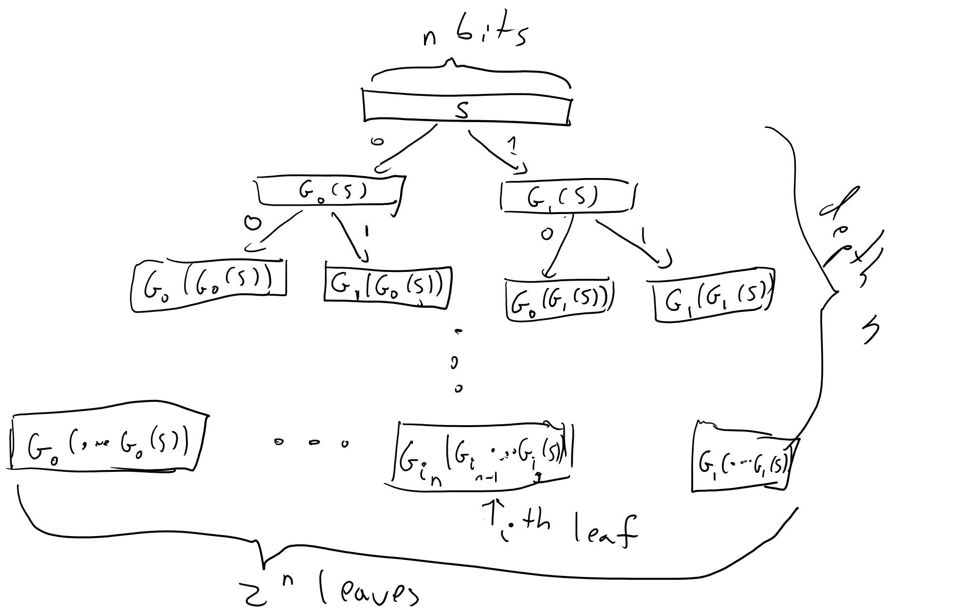
Proof: If the PRG Conjecture is true then in particular by the length extension theorem there exists a PRG \(G:{\{0,1\}}^n\rightarrow{\{0,1\}}\) that maps \(n\) bits into \(2n\) bits. Let’s denote \(G(s)=G_0(s)\circ G_1(s)\) where \(\circ\) denotes concatenation. That is, \(G_0(s)\) denotes the first \(n\) bits and \(G_1(s)\) denotes the last \(n\) bits of \(G(s)\).

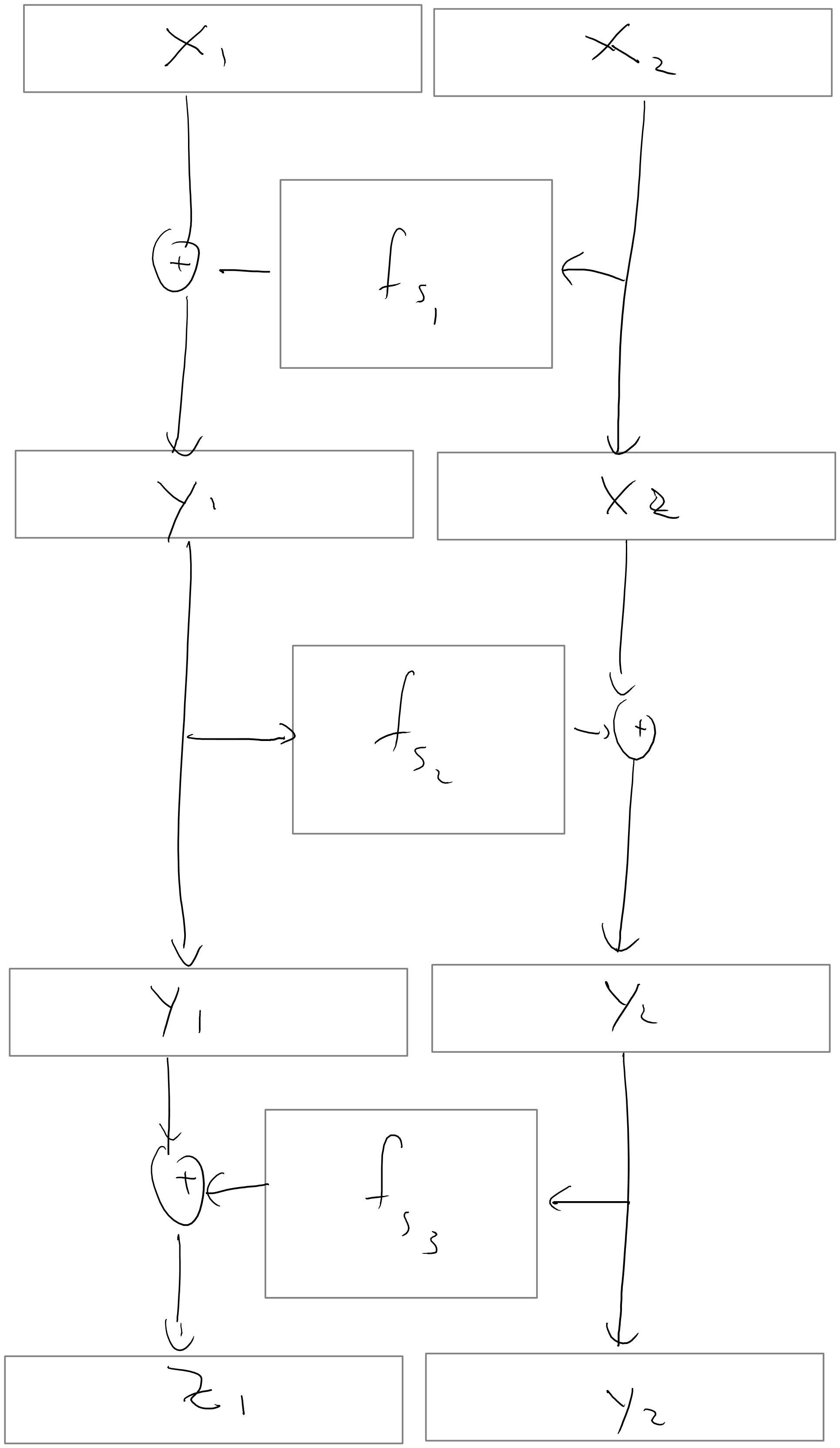
For \(i\in{\{0,1\}}^n\), we define \(f_s(i)\) as \[G_{i_n}(G_{i_{n-1}}(\cdots G_{i_1}(s))).\]

This might be a bit hard to parse and is easier to understand via a figure:

The construction of a pseudorandom function from a pseudorandom generator can be illustrated by a depth \(n\) binary tree. The root is labeled by the seed \(s\) and for every internal node \(v\) labeled by a strong \(x\in{\{0,1\}}^n\), we label the two children of \(v\) by \(G_0(x)\) and \(G_1(x)\) respectively. The output of the function \(f_s\) on input \(i\) is the label of the \(i^{th}\) leaf.

By the definition above we can see that to evaluate \(f_s(i)\) we need to evaluate the pseudorandom generator \(n\) times on inputs of length \(n\), and so if the pseudorandom generator is efficiently computable then so is the pseudorandom function. Thus, “all” that’s left is to prove that the construction is secure and this is the heart of this proof.

I’ve mentioned before that the first step of writing a proof is convincing yourself that the statement is true, but there is actually an often more important zeroth step which is understanding what the statement actually means. In this case what we need to prove is the following:

Given an adversary \(A\) that can distinguish in time \(T\) a black box for \(f_s(\cdot)\) from a black-box for a random function with advantage \(\epsilon\), we need to come up with an adversary \(D\) that can distinguish in time \(poly(T)\) an input of the form \(G(s)\) (where \(s\) is random in \({\{0,1\}}^n\)) from an input of the form \(y\) where \(y\) is random in \({\{0,1\}}^{2n}\) with bias at least \(\epsilon/poly(T)\).

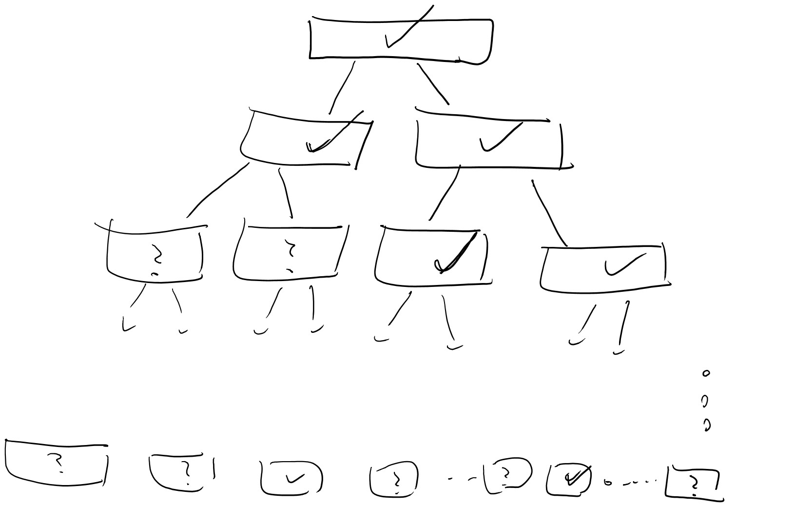
Let us consider the “lazy evaluation” implementation of the black box for \(A\) illustrated in the following figure:

In the “lazy evaluation” implementation of the black box to the adversary, we label every node in the tree only when we need it. In this figure check marks correspond to nodes that have been labeled and question marks to nodes that are still unlabeled.

That is, at every point in time there are nodes in the full binary tree that are labeled and nodes which we haven’t yet labeled. When \(A\) makes a query \(i\), this query corresponds to the path \(i_1\ldots i_n\) in the tree. We look at the lowest (furthest away from the root) node \(v\) on this path which has been labeled by some value \(y\), and then we continue labelling the path from \(v\) downwards until we reach \(i\). That is, we label the two children of \(v\) by \(G_0(y)\) and \(G_1(y)\), and then if the path \(i\) involves the first child then we label its children by \(G_0(G_0(y))\) and \(G_1(G_0(y))\), and so on and so forth.

When the adversary queries \(i\), the oracle takes the path from \(i\) to the root and computes the generator on the minimum number of internal nodes that is needed to obtain the label of the \(i^{th}\) leaf

A moment’s thought shows that this is just another (arguably cumbersome) way to describe the oracle that simply computes the map \(i\mapsto f_s(i)\). And so the experiment of running \(A\) with this oracle produces precisely the same result as running \(A\) with access to \(f_s(\cdot)\). Note that since \(A\) has running time at most \(T\), the number of times our oracle will need to label an internal node is at most \(T' \leq 2nT\) (since we label at most \(2n\) nodes for every query \(i\)).

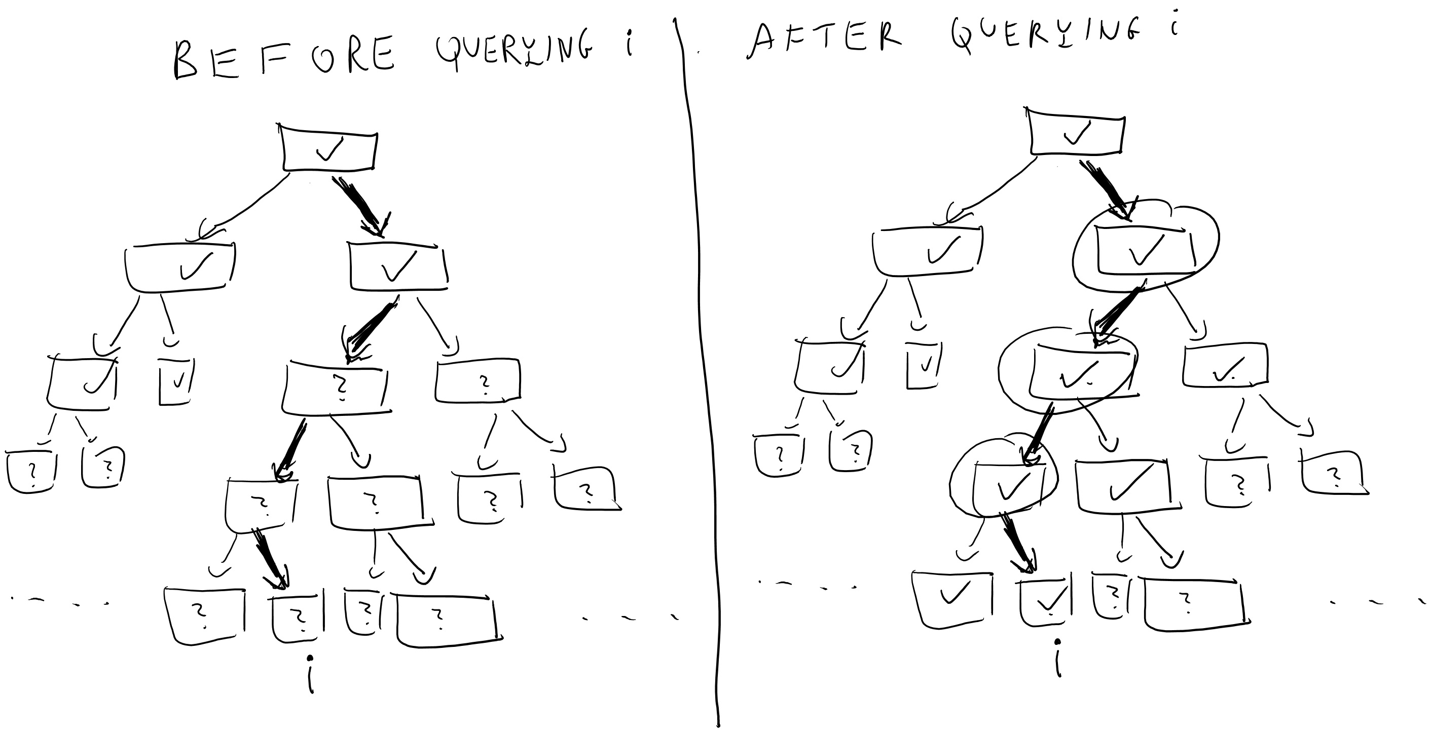
We now define the following \(T'\) hybrids: in the \(j^{th}\) hybrid, we run this experiment but in the first \(j\) times the oracle needs to label internal nodes, then instead of labelling the \(b^{th}\) child of \(v\) by \(G_b(y)\) (where \(y\) is the label of \(v\)), the oracle simply labels it by a random string in \({\{0,1\}}^n\).

Note that the \(0^{th}\) hybrid corresponds to the case where the oracle implements the function \(i\mapsto f_s(i)\) will in the \(T'^{th}\) hybrid all labels are random and hence the oracle implements a random function. By the hybrid argument, if \(A\) can distinguish between the \(0^{th}\) hybrid and the \(T'^{th}\) hybrid with bias \(\epsilon\) then there must exists some \(j\) such that it distinguishes between the \(j^{th}\) hybrid and the \(j+1^{st}\) hybrid with bias at least \(\epsilon/T'\). We will use this \(j\) and \(A\) to break the pseudorandom generator.

We can now describe our distinguisher \(D\) for the pseudorandom generator. On input a string \(y\in{\{0,1\}}^{2n}\) \(D\) will run \(A\) and the \(j^{th}\) oracle inside its belly with one difference- when the time comes to label the \(j^{th}\) node, instead of doing this by applying the pseudorandom generator to the label of its parent \(v\) (which is what should happen in the \(j^{th}\) oracle) it uses its input \(y\) to label the two children of \(v\).

Now, if \(y\) was completely random then we get exactly the distribution of the \(j+1^{st}\) oracle, and hence in this case \(D\) simulates internally the \(j+1^{st}\) hybrid. However, if \(y=G(s)\) for a random \(s\in{\{0,1\}}^n\) it might not be obvious if we get the distribution of the \(j^{th}\) oracle, since in that oracle the label for the children of \(v\) was supposed to be the result of applying the pseudorandom generator to the label of \(v\) and not to some other random string. However, because \(v\) was labeled before the \(j^{th}\) step then we know that it was actually labeled by a random string. Moreover, since we use lazy evaluation we know that step \(j\) is the first time where we actually use the value of the label of \(v\). Hence, if at this point we resampled this label and used a completely independent random string then the distribution would be identical . Hence if \(y=G(U_n)\) then \(D\) actually does simulate the distribution of the \(j^{th}\) hybrid in its belly, and thus if \(A\) had advantage \(\epsilon\) in breaking the PRF \(\{ f_s \}\) then \(D\) will have advantage \(\epsilon/T'\) in breaking the PRG \(G\) thus obtaininer a contradiction. QED

This proof is ultimately not very hard but is rather confusing. I urge you to also look at the proof of this theorem as is written in Section 7.5 (pages 265-269) of the KL book.

PRF’s in practice: While this construction reassures us that we can rely on the existence of pseudorandom functions even on days where we remember to take our meds, this is not the construction people use when they need a PRF in practice because it is still somewhat inefficient, making \(n\) calls to the underlying pseudorandom generators. There are constructions (e.g., HMAC) based on hash functions that require stronger assumptions but can use as few as two calls to the underlying function. We will cover these constructions when we talk about hash functions and the random oracle model.

Securely encrypting many messages - chosen plaintext security

Let’s get back to our favorite task of encryption . We seemed to have nailed down the definition of secure encryption, or did we? Our current definition requires talks about encrypting a single message, but this is not how we use encryption in the real world. Typically, Alice and Bob (or Amazon and Boaz) setup a shared key and then engage in many back and forth messages between one another.

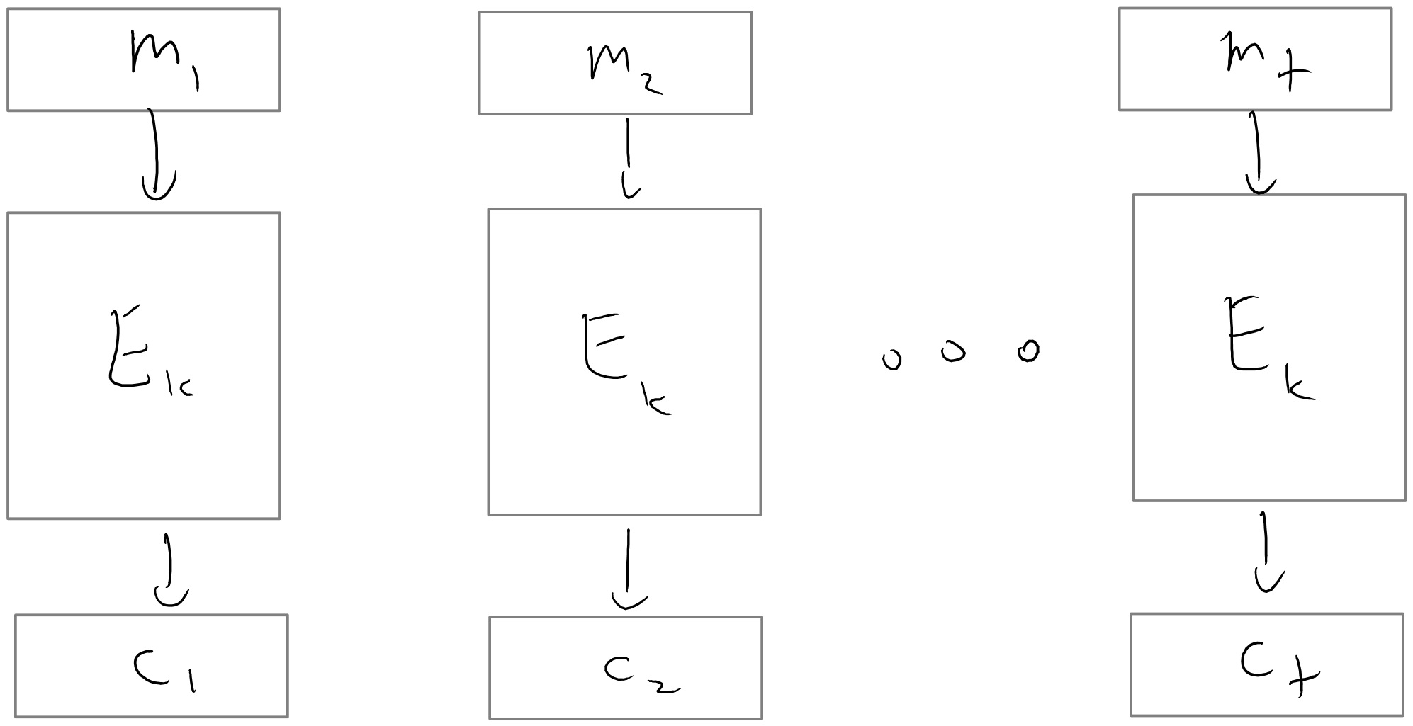
At first, we might thing that this issue of a single long message vs. many short ones is merely a technicality. After all, if Alice wants to send a sequence of messages \((m_1,m_2,\ldots,m_t)\) to Bob, she can simply treat them as a single long message. Moreover, the way that stream ciphers work, Alice can compute the encryption for the first few bits of the message she decides what will be the next bits and so she can send the encryption of \(m_1\) to Bob and later the encryption of \(m_2\). There is some truth to this sentiment, but there is also an issue that it misses. For Alice and Bob to encrypt messages in this way, they must maintain a syncrhonized shared state. If the message \(m_1\) was dropped by the network, then Bob would not be able to decrypt correctly the encryption of \(m_2\).

There is another way in which treating many messages as a single tuple is unsatisfactory. In real life, Eve might be able to have some impact on what messages Alice encrypts. For example, the Katz-Lindell book describes several instances in world war II where Allied forces made particular military manouvers for the sole purpose of causing the axis forces to send encryptions of messages of the Allies’ choosing. For a more modern example, today Google uses encryption for all of its search traffic including (for the most part) the ads that are displayed on the page. But this means that an attacker, by paying Google, can cause it to encrypt arbitrary text of their choosing. This kind of attack, where Eve chooses the message she wants to be encrypted is called a chosen plaintext attack. You might think that we are already covering this with our current definition that requires security for every pair of messages and so in particular this pair could chosen by Eve. However, in the case of multiple messages, we would want to allow Eve to be able to choose \(m_2\) after she saw the encryption of \(m_1\).

All that leads us to the following definition, which is a strenghtening of our definition of computational security:

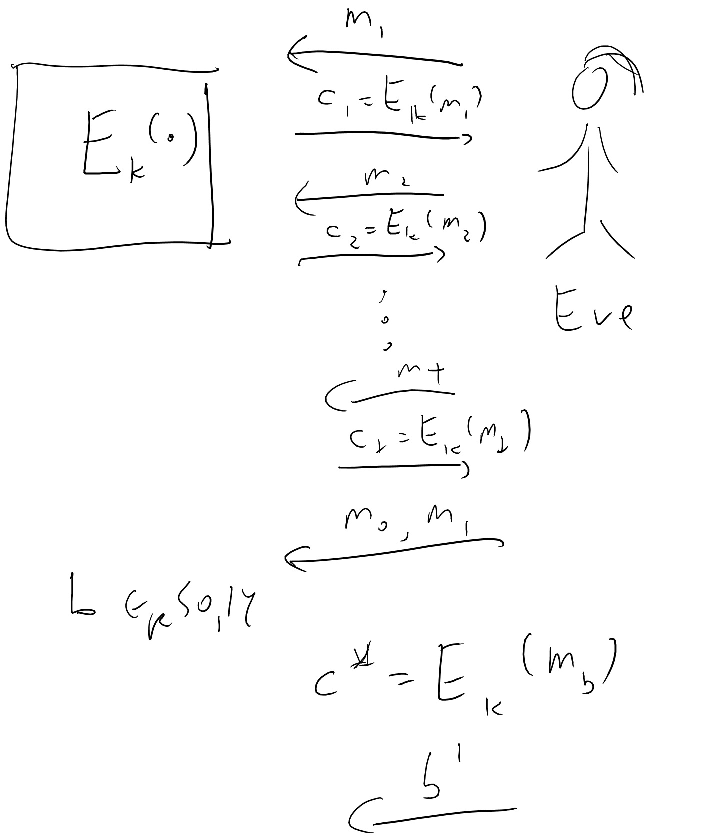
Definition (CPA security): An encryption scheme \((E,D)\) is secure against chosen plaintext attack (CPA secure) if for every polynomial time \(Eve\), Eve wins with probability at most \(1/2+negl(n)\) in the game defined below:

1. The key \(k\) is chosen at random in \({\{0,1\}}^n\) and fixed.

2. Eve gets the length of the key \(1^n\) as input.¹

3. Eve interacts with \(E\) for \(t=poly(n)\) rounds as follows: in the \(i^{th}\) round, Eve chooses a message \(m_i\) and obtains \(c_i= E_k(m_i)\).

4. Then Eve chooses two messages \(m_0,m_1\), and gets \(c^* = E_k(m_b)\) for \(b{\leftarrow_R\;}{\{0,1\}}\).

5. Eve wins if she outpus \(b\).

In the CPA game, Eve interacts with the encryption oracle and at the end chooses \(m_0,m_1\), gets an encryption \(c^*=E_k(m_b)\) and outputs \(b'\). She wins if \(b'=b\)

Note that our previous notion of computational security corresponded to the case that we skipped Step 3 above. Hence this new notion implies the previous one. It turns out that it is strictly stronger, in the sense that without modification, our stream ciphers cannot be CPA secure. In fact, we have a stronger, and intially somewhat surprising theorem:

Theorem: There is no CPA secure \((E,D)\) where \(E\) is deterministic.

Proof: The proof is very simple: Eve will only use a single round of interacting with \(E\) where she will ask for the encryption \(c_1\) of \(0^\ell\). In the second round, Eve will choose \(m_0=0^{\ell}\) and \(m_1=1^{\ell}\), and get \(c^*=E_k(m_b)\) she wil then output \(0\) if and only if \(c^*=c_1\). QED

This proof is so simple that you might think it shows a problem with the definition, but it is actually a real problem with security. If you encrypt many messages and some of them repeat themselves, it is possible to get significant information by seeing the repetition pattern (que the XKCD cartoon again):

Insecurity of deterministic encryption

To avoid this issue we need to use probabilistic encryption.² But how do we do that? Here is a simple CPA secure scheme:

Theorem: Suppose that \(\{ f_s \}\) is a PRF collection where \(f_s:{\{0,1\}}^n\rightarrow{\{0,1\}}^\ell\), then the following is a CPA secure encryption scheme: \(E_s(m)=(r,f_s(r)\oplus m)\) and \(D_s(r,z)=f_s(r)\oplus z\).

Proof: I leave to you to verify that \(D_s(E_s(m))=m\). I need to show the CPA security property. As is usual in PRF-based constructions, we first show that this scheme will be secure if \(f_s\) was an actually random function, and then use that to derive security.

Consider the game above when played with a completely random function and let \(r_i\) be the random string chosen by \(E\) in the \(i^{th}\) round and \(r^*\) the string chosen in the last round. We start with the following simple but crucial claim:

Claim: The probability that \(r^*=r_i\) for some \(i\) is at most \(T/2^n\).

Proof: For any particular \(i\), since \(r^*\) is chosen independently of \(r_i\), the probability that \(r^*=r_i\) is \(2^{-n}\). Hence the claim follows from the union bound. QED

Given this claim we know that with probability \(1-T/2^n\) (which is \(1-negl(n)\)), the string \(r^*\) is distinct from any string that was chosen before. This means that by the lazy evaluation principle, if \(f_s(\cdot)\) is a completely random function then the value \(f_s(r^*)\) can be thought of as being chosen at random in the final round independently of anything that happened before. But then \(f_s(r^*)\oplus m_b\) amounts to simply using the one-time pad to encrypt \(m_b\). That is, the distributions \(f_s(r^*)\oplus m_0\) and \(f_s(r^*)\oplus m_1\) (where we think of \(r^*,m_0,m_1\) as fixed and the randomness comes from the choice of the random function \(f_s(\cdot)\)) are both equal to the uniform distribution \(U_n\) over \({\{0,1\}}^n\) and hence Eve gets absolutely no information about \(b\).

This shows that if \(f_s(\cdot)\) was a random function then Eve would win the game with probability at most \(1/2\). Now if we have some efficient Eve that wins the game with probability at least \(1/2+\epsilon\) then we can build an adversary \(A\) for the PRF that will run this entire game with black box access to \(f_s(\cdot)\) and will output \(1\) if and only if Eve wins. By the argument above, there would be a difference of at least \(\epsilon\) in the probability it outputs \(1\) when \(f_s(\cdot)\) is random vs when it is pseudorandom, hence contradicting the security property of the PRF. QED

Pseudorandom permutations / block ciphers

Now that we have pseudorandom functions, we might get greedy and want such functions with even more magical properties. This is where the notion of pseudorandom permutations comes in.

Definition: A collection of functions \(\{ f_s \}\) where \(f_s:{\{0,1\}}^\ell\rightarrow{\{0,1\}}^\ell\) is called a pseudorandom permutation (PRP) collection if (a) it is a pseudorandom function collection, (b) every function \(f_s\) is a permutation of \({\{0,1\}}^n\) (i.e., a one to one and onto map), and (c) there is an efficient algorithm that on input \(s,y\) returns \(f_s^{-1}(y)\).

As usual with a new concept, we want to know whether it is possible to achieve and is useful. The former is established by the following theorem:

Theorem: If the PRG conjecture holds then there exists a pseudorandom permutation collection.

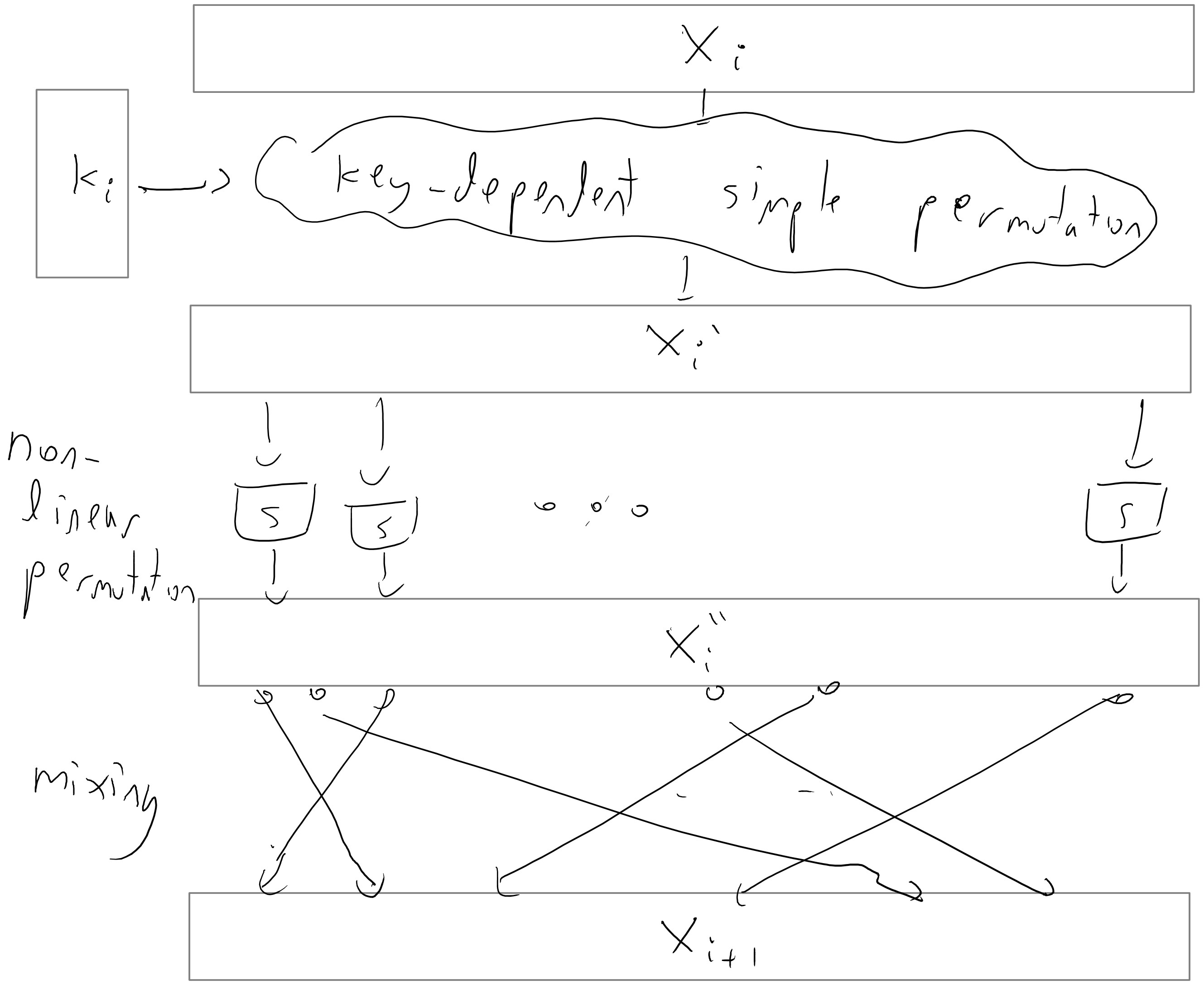
We will not show the proof of this theorem here, but just show a figure of the construction:

We build a PRP \(p\) on \(2n\) bits from three PRFs \(f_{s_1},f_{s_2},f_{s_3}\) on \(n\) bits by letting \(p_{s_1,s_2,s_3}(x_1,x_2)=(z_1,y_2)\) where \(y_1 = x_1 \oplus f_{s_1}(x_2)\), \(y_2 = x_2 \oplus f_{s_2}(y_1)\) and \(z_1 = f_{s_3}(y_2) \oplus y_1\).

The more common name for a pseudorandom permutation is block cipher (though typically block ciphers are expected to meet additional security properties on top of being PRPs). The constructions for block ciphers used in practice typically don’t follow this theorem (though they use some of the ideas) but rather build these directly.

One of the first modern block ciphers was the Digital Encryption Standard (DES) constructed by IBM in the 1970’s. It is a fairly good cipher- to this day, as far as we know, it provides a pretty good number of security bits compared to its key. The trouble is that its key is only \(56\) bits long, which is no longer outside the reach of modern computing power. (It turned out that subtle variants of DES are far less secure and fall prey to a technique known as differential cryptanalysis; the IBM designers of DES were aware of this technique but kept it secret at the behest of the NSA.)

Between 1997 and 2001, the U.S. national institute of standards (NIST) ran a competition to replace DES which resulted in the adoption of the block cipher Rijndael as the new advanced encryption standard (AES). It has a block size of 128 bits and a key size of 128, 196, or 256 bits.

The actual construction of AES (or DES for that matter) is not extremely illuminating, but let us say a few words about the general principle behind many block ciphers. They are typically constructed by repeating one after the other a number of very simple permutations. Each such iteration is called a round. If there are \(t\) keys, then the key \(k\) is typically expanded into a \(t\) tuple of keys \(*k_1,\ldots,k_t)\) via some pseudorandom generator known as the key scheduling algorithm and then the key \(k_i\) is used in the \(i^{th}\) round. Each round is typically composed of several components: there is a “key mixing component” that performs some simple permutation based on the key (often as simply as XOR’ing the key), there is a “mixing component” that mixes the bits of the block so that bits that were intially nearby don’t stay close to one another, and then there is some non-linear component (often obtained by applying some simple non-linear functions known as “S boxes” to each small block of the input) that ensures that the overall cipher will not be an affine function. Each one of these operations is an easily reversible operations, and hence decrypting the cipher simply involves running the rounds backwards.

A typical round of a block cipher, \(k_i\) is the \(^{th}\) round key, \(x_i\) is the block before the \(i^{th}\) round and \(x_{i+1}\) is the block at the end of this round.

Encryption modes

How do we use a block cipher to actually encrypt traffic? Well we could use it as a PRF in the construction above, but in practice people use other ways.

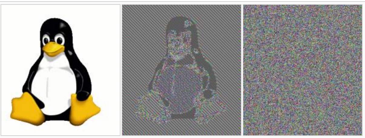
The most natural approach would be that to encrypt a message \(m\), we simply use \(p_s(m)\) where \(\{ p_s \}\) is the PRP/block cipher. This is known as the electronic code book (ECB) mode of a block cipher. Note that we can easily decrypt since we can compute \(p_s^{-1}(m)\). However, this is a deterministic encryption and hence cannot be CPA secure. Moreover, this is actually a real problem of security on realistic inputs.

In the Electronic Codebook (ECB) mode every message is encrypted deterministically and independently

An encryption of the Linux penguin (left image) using ECB mode (middle image) vs CBC mode (right image). The ECB encryption is insecure as it reveals much structure about the original image. Image taken from Wikipedia.

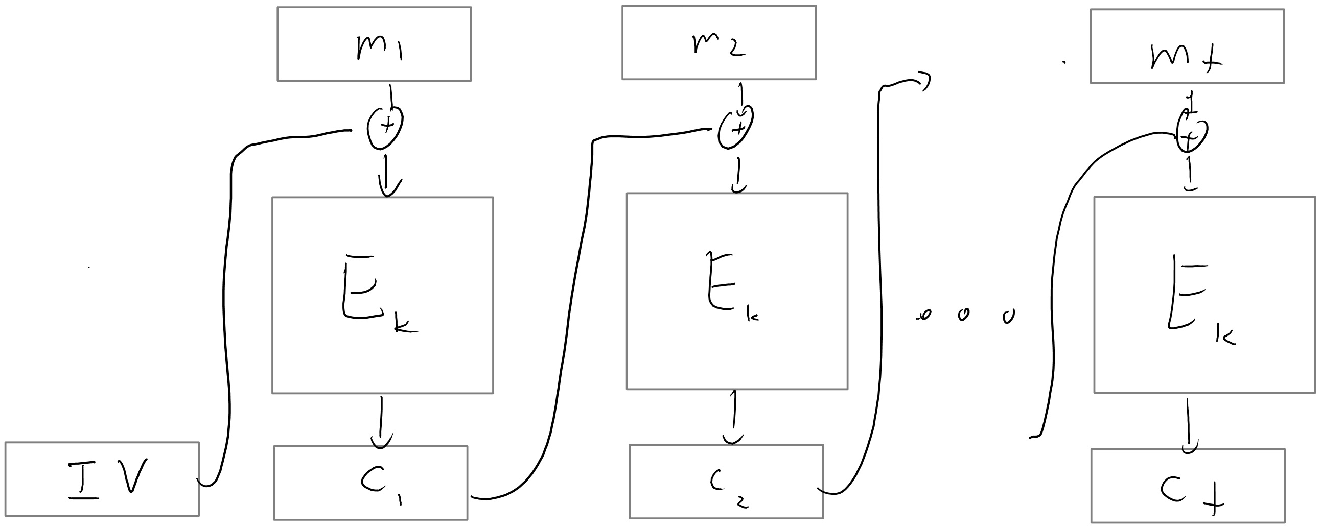
A more secure way to use a block cipher to encrypt is the cipher block chaining mode where we XOR every message with the previous ciphertext. Note that if we lose a block to traffic in the CBC mode then we are unable to decrypt the next block, but can recover from that point onwards.

In the Cypher-Block-Chaining (CBC) the encryption of the previous message is XOR’ed into the current message prior to encrypting. The first message is XOR’ed with an initialization vector (IV) that if chosen randomly, ensures CPA security.

It turns out that using this mode with a random IV can yield CPA security, though one has to be careful in how you go about it, see the exercises.

In the output feedback mode we encrypt the all zero string using CBC mode to get a sequence \((y_1,y_2,\ldots)\) of pseudorandom outputs that we can use as a stream cipher.

Perhaps the simplest mode is counter mode where we convert a block cipher to a stream cipher by using the stream \(p_k(IV),p_k(IV+1),p_k(IV+2),\ldots\) where \(IV\) is a random string in \({\{0,1\}}^n\) which we identify with \([2^n]\) (and perform addition modulo \(2^n\)) . For a modern block cipher this should be no less secure than CBC or OFB and has advantages that we can easily compute it in parallel.

A fairly comprhensive study of the different modes of block ciphers is in this document by Rogaway. His conclusion is that if we simply consider CPA security (as opposed to the stronger notions we’ll see in the next lecture) then counter mode is the best choice, but CBC, OFB and CFB are widely implemented due to legacy reasons. ECB should not be used (except as a building block as part of a construction achieving stronger security).1