Length extension for pseudorandom generators
~ MathDefs ~
CS 127: Cryptography / Boaz Barak
Reading: Katz-Lindell Section 3.3, Boneh-Shoup Chapter 3
The nature of randomness has troubled philosophers, scientists, statisticians and laypeople for many years.1 Over the years people have given different answers to the question of what does it mean for data to be random, and what is the nature of probability. The movements of the planets initially looked random and arbitrary, but then the early astronomers managed to find order and make some predictions on them. Similarly we have made great advances in predicting the weather, and probably will continue to do so in the future. So, while these days it seems as if the event of whether or not it will rain a week from today is random, we could imagine that in some future we will be able to perfectly predict it. Even the canonical notion of a random experiment- tossing a coin - turns out that it might not be as random as you’d think, with about a 51% chance that the second toss will have the same result as the first one. (Though see also this experiment.) It is conceivable that at some point someone would discover some function \(F\) that given the first 100 coin tosses by any given person can predict the value of the 101\(^{th}\).2 Note that in all these examples, the physics underlying the event, whether it’s the planets’ movement, the weather, or coin tosses, did not change but only our powers to predict them. So to a large extent, randomness is a function of the observer, or in other words
If a quantity is hard to compute, it might as well be random.
Much of cryptography is about trying to make this intuition more formal, and harnessing it to build secure systems. The basic object we want is the following:
Definition (Pseudo random generator): An efficiently computable function \(G:{\{0,1\}}^n\rightarrow{\{0,1\}}^\ell\) is a pseudorandom generator if \(\ell>n\) and \(G(U_n) \approx U_\ell\) where \(U_t\) denotes the uniform distribution on \({\{0,1\}}^t\).
Note that the requirement that \(\ell>n\) is crucial to make this notion non-trivial, as for \(\ell=n\) the function \(G(x)=x\) clearly satisfies that \(G(U_n)\) is identical to (and hence indistinguishable from) the distribution \(U_n\). (Make sure that you understand this last statement!) However, for \(\ell>n\) this is no longer trivial at all, and in particular if we didn’t restrict the running time of \(Eve\) then no such pseudo-random generator would exist:
Lemma: Suppose that \(G:{\{0,1\}}^n\rightarrow{\{0,1\}}^{n+1}\). Then there exists an (inefficient) algorithm \(Eve:{\{0,1\}}^{n+1}\rightarrow{\{0,1\}}\) such that \({\mathbb{E}}[ Eve(G(U_n)) ]=1\) but \({\mathbb{E}}[ Eve(U_{n+1})] \leq 1/2\).
Proof: On input \(y\in{\{0,1\}}^{n+1}\), \(Eve\) go over all possible \(x\in{\{0,1\}}^n\) and will output \(1\) if and only if \(y=G(x)\) for some \(x\). Clearly \({\mathbb{E}}[ Eve(G(U_n)) ] =1\). However, the set \(S =\{ G(x) : x\in {\{0,1\}}^n \}\) on which Eve outputs \(1\) has size at most \(2^n\), and hence a random \(y{\leftarrow_{\tiny R}}U_n\) will fall in \(S\) with probability at most \(1/2\). QED
It is not hard to show that if \(P=NP\) then the above algorithm Eve can be made efficient, and hence in particular at the moment we do not know how to prove the existence of pseudorandom generators. Nevertheless they are widely believed to exist and hence we make the following conjecture:
Conjecture (The PRG conjecture): For every \(n\), there exists a pseudorandom generator \(G\) mapping \(n\) bits to \(n+1\) bits.
As was the case for the cipher conjecture, and any other conjecture, there are two natural questions regarding the PRG conjecture: why should we believe it and why should we care. Fortunately, the answer to the first question is simple: it is known that the cipher conjecture implies the PRG conjecture, and hence if we believe the former we should believe the latter. (The proof is highly non trivial and we may not get to see it in this course.) As for the second question, we will see that the PRG conjecture implies a great number of useful cryptographic tools, including the cipher conjecture. We start by showing that once we can get to an output that is one bit longer than the input, we can in fact obtain any number of bits.
Theorem (length extension for PRG’s): Suppose that the PRG conjecture is true. Then for every polynomial \(t(n)\), there exists a pseudorandom generator mapping \(n\) bits to \(t(n)\) bits.
Proof: The proof of this theorem is very similar to the length extension theorem for ciphers, and in fact this theorem can be used to give an alternative proof for the former theorem.
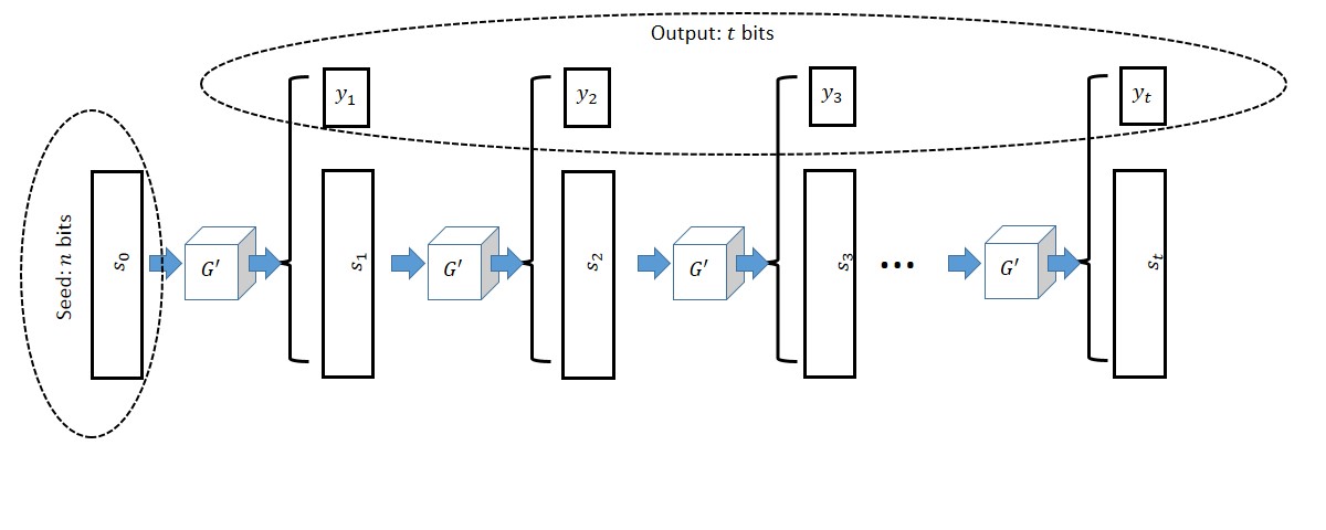
The construction is illustrated in the figure below:
Length extension for pseudorandom generators
We are given a pseudorandom generator \(G'\) mapping \(n\) bits into \(n+1\) bits and need to construct a pseudorandom generator \(G\) mapping \(n\) bits to \(t=t(n)\) bits for some polynomial \(t(\cdot)\). The idea is that we maintain a state of \(n\) bits, which are originally our input seed3 \(s_0\), and at the \(i^{th}\) step we use \(G'\) to map \(s_{i-1}\) to the \(n+1\)-long bit string \((s_i,y_i)\), output \(y_i\) and keep \(s_i\) as our new state. To prove the security of this construction we need to show that the distribution \(G(U_n) = (y_1,\ldots,y_t)\) is computationally indistinguishable from the uniform distribution \(U_t\). As usual, we will use the hybrid argument. For \(i\in\{0,\ldots,t\}\) we define \(H_i\) to be the distribution where the first \(i\) bits chosen at uniform, whereas the last \(t-i\) bits are computed as above. Namely, we choose \(s_i\) at random in \(\zo^n\) and continue the computation of \(y_{i+1},\ldots,y_t\) from the state \(s_i\). Clearly \(H_0=G(U_n)\) and \(H_t=U_t\) and hence by the triangle inequality it suffices to prove that \(H_i \approx H_{i+1}\) for all \(i\in\{0,\ldots,t-1\}\). We illustrate these two hybrids in the following figure:
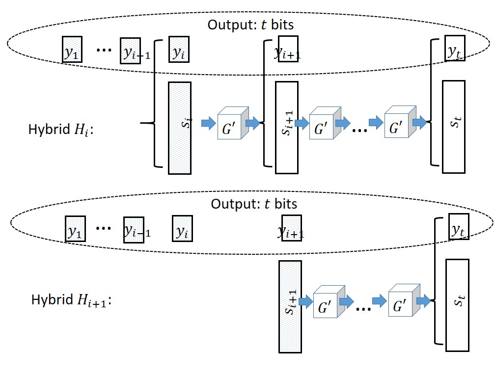
Hybrids \(H_i\) and \(H_{i+1}\)— dotted boxes refer to values that are chosen independently and uniformly at random
Suppose otherwise, that there exists some adversary \(Eve\) such that \(\left| \E[Eve(H_i)] - \E[Eve(H_{i+1})] \right| \geq \epsilon\) for some non-negligible \(\epsilon\). We will build from \(Eve\) an adversary \(Eve'\) breaking the security of the pseudorandom generator \(G'\).
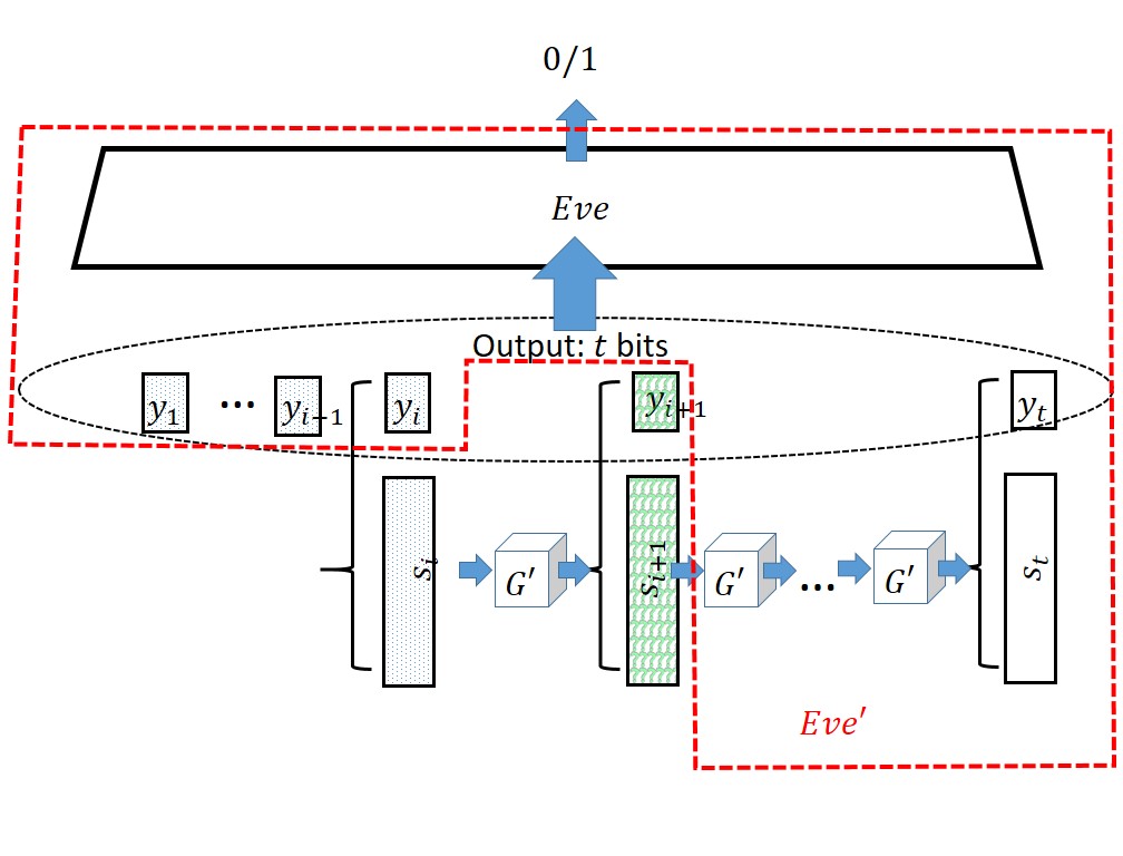
Building an adversary \(Eve'\) for \(G'\) from an adversary \(Eve\) distinguishing \(H_i\) and \(H_{i+1}\). The boxes marked with questions marks are those that are random or pseudorandom depending on whether we are in \(H_i\) or \(H_{i+1}\). Everything inside the dashed red lines is simulated by \(Eve'\) that gets as input the \(n+1\)-bit string \((s_{i+1},y_{i+1})\).
On input an \(n+1\) string \(y\), \(Eve'\) will interpret \(y\) as \((s_{i+1},y_{i+1})\), choose \(y_1,\ldots,y_i\) randomly and compute \(y_{i+2},\ldots,y_t\) as in our pseudorandom generator’s construction. \(Eve'\) will then feed \((y_1,\ldots,y_t)\) to \(Eve\) and output whatever \(Eve\) does. Clearly, \(Eve'\) is efficient if \(Eve\) is. Moreover, one can see that if \(y\) was random then \(Eve'\) is feeding \(Eve\) with an input distributed according to \(H_{i+1}\) while if \(y\) was for the form \(G(s)\) for a random \(s\) then \(Eve'\) will feed \(Eve\) with an input distributed according to \(H_i\). Hence we get that \(| \E[ Eve'(G(U_n))] - \E[Eve'(U_{n+1})] | \geq \epsilon\) contradicting the security of \(G'\) QED.
Aside: Unpredictablity and indistinguishability- an alternative approach for proving the length extension theorem. The notion that being random is the same as being “unpredictable” can be formalized as follows. One can show that a random variable \(X\) over \(\zo^n\) is pseudorandom if and only every efficient algorithm \(A\) succeeds in the following experiment with probability at most \(1/2+negl(n)\): \(A\) is given \(i\) chosen at random in \(\{0,\ldots,n-1\}\) and \(x_1,\ldots,x_i\) where \((x_1,\ldots,x_n)\) is drawn from \(X\) and wins if it outputs \(x_{i+1}\). It is a good optional exercise to prove this, and to use that to give an alternative proof of the length extension theorem.
We now show a connection between our two notions:
Theorem: If the PRG conjecture is true then so is the cipher conjecture.
We note that it turns out that the converse direction is also true, and hence these two conjectures are equivalent, though we will probably not show the (quite non-trivial) proof of this fact in this course. (We might show some a weaker version of this harder direction later in the course.)
Proof: The construction is actually quite simple, recall that the one time pad is a perfectly secure cipher but its only problem was that to encrypt an \(n+1\) long message it needed an \(n+1\) long bit key. Now using a pseudorandom generator, we can map an \(n\)-bit long key into an \(n+1\)-bit long string that looks random enough that we could use it as a key for the one-time pad. That is, our cipher will look as follows:
\[ E_k(m) = G(k) \oplus m \]
and
\[ D_k(c) = G(k) \oplus c \]
Just like in the one time pad, \(D_k(E_k(m)) = G(k) \oplus G(k) \oplus m = m\). Moreover, the encryption and decruption algorithms are clearly efficient and so the only thing that’s left is to prove security or that for every \(m,m' E_{U_n}(m) \approx E_{U_n}(m')\). We show this by proving the following claim:
Claim: For every \(m\in{\{0,1\}}^{n+1}\), \(E_{U_n}(m) \approx U_{n+1} \oplus m\).
The claim implies the security of the scheme, since it means that \(E_{U_n}(m)\) is indistinguishable from the one-time-pad encryption of \(m\), which is identically distributed to the one-time pad encryption of \(m'\) which (by another application of the claim) is indistinguishable from \(E_{U_n}(m')\) and so the theorem follows from the triangle inequality. Thus all that’s left is to prove the claim:
Proof of claim: Suppose that there was an efficient adversary \(Eve'\) such that
\[ \left| {\mathbb{E}}[ Eve'(G(U_n)\oplus m)] - {\mathbb{E}}[ Eve'(U_{n+1}\oplus m) ] \right| \geq \epsilon \]
for some non-negligible \(\epsilon=\epsilon(n)>0\). Then the adversary \(Eve\) defined as \(Eve(y) = Eve'(y\oplus m)\) would be also efficient and would break the security of the PRG with non-negligible success. QED
Note that if the PRG outputs \(t(n)\) bits instead of \(n+1\) then we automatically get an encryption scheme with \(t(n)\) long message length. In fact, in practice if we use the length extension for PRG’s, we don’t need to decide on the length of messages in advance. Every time we need to encrypt another bit (or another block) \(m_i\) of the message, we run the basic PRG to update our state and obtain some new randomness \(y_i\) that we can XOR with the message and ouput. Such constructions are known as stream ciphers in the literature. In fact, in most of the practical literature the mame stream cipher is used both for the pseudorandom generator itself, as well as for the encryption scheme that is obtained by combining it with the one-time pad.
Aside: Using pseudorandom generators for coin tossing over the phone. The following is a cute application of pseudorandom generators. Alice and Bob want to toss a fair coin over the phone. They use a pseudorandom generator \(G:\zo^b\rightarrow\zo^{3n}\). Alice will send \(z\getsr\zo^{3n}\) to Bob, Bob picks \(s\getsr\zo^n\) and with probability \(1/2\) sends \(G(s)\) (case I) and with probability \(1/2\) sends \(G(s)\oplus z\) (case II). Alice then picks a random \(b\getsr\zo\) and sends it to Bob. Bob then reveals what he sent in the previous stage and if it was case I, their output is \(b\), and if it was case II, their output is \(1-b\).
So far we have made the conjectures that objects such as ciphers and pseudorandom generators exist, without giving any hint as to how they would actually look like. While as mentioned above, we do not know how to prove that any particular function is a pseudorandom generators, it turns out that there are quite simple candidates for such functions, though care must be taken in constructing them. We now consider candidates for functions that maps \(n\) bits to \(n+1\) bits (or more generally \(n+c\) for some constant \(c\) ) and look at least somewhat “randomish”. As these constructions are typically used as a basic component for obtaining a longer length PRG via the length extension theorem, we will think of these pseudorandom generators as mapping a string \(s\in\zo^n\) representing the current state into a string \(s’\in\zo^n\) representing the new state as well as a string \(b\in\zo^c\) representing the current output. See also Section 6.1 in Katz-Lindell and (for greater depth) Sections 3.6-3.9 in the Boneh-Shoup book.
One of the simplest ways to generate a “randomish” digit from an \(n\) digit number is to use a checksum - some linear combination of the digits, as is the cyclic redundancy check or CRC. This motivates the notion of a linear feedback shift register generator (LFSR): if the current state is \(s\in\zo^n\) then the output is \(f(s)\) where \(f\) is a linear function (modulo 2) and the new state is obtained by right shifting the previous state and putting \(f(s)\) at the leftmost location. That is, \(s’_1 = f(s)\) and \(s’_i = s_{i-1}\) for \(i\in\{2,\\ldots,n\}\).
LFSR’s have several good properties- if the function \(f(\cdot)\) is chosen properly then they can have very long periods (i.e., it takes \(2^n\) steps until the state repeats itself), though that also holds for the simple “counter” generator who simply treats the state as a number in \(\{0,\ldots,2^n-1\}\) and increments it at every stage, outputting the least significant digit. They also have the property that every individual bit is equal to \(0\) or \(1\) with probability exactly half (the counter generator also shares this property) as well as (if the function is selected properly) that every two bits are independent from one another (the counter fails badly here - the least significant bits between two consecutive states always flip). (Showing the last facts is a great optional exercise.)
There is a more general notion of a linear generator where the new state can be any invertible linear transformation of the previous state. That is, we interpret the state \(s\) as an element of \(\Z_q^t\) for some integers \(q,t\),4 and let \(s’=F(s)\) and the output \(b=G(s)\) where \(F:\Z_q^t\rightarrow\Z_q^t\) and \(G:\Z_q^t\rightarrow\Z_q\) are some invertible linear transformation (modulo \(q\)). This includes as a special case the linear congruential generator where \(t=1\) and the map \(F(s)\) corresponds to taking \(as \pmod{q}\) where \(a\) is number co-prime to \(q\).
All these generators are unfortunately insecure due to the great bane of cryptography- the Gaussian Elimination algorithm. This algorithm (and some generalizations and related algorithms such as Euclid’s extended g.c.d algorithm and the LLL lattice reduction algorithm) has been used time and again to break candidate cryptographic constructions.
The unfortunate theorem for cryptography (Author(s) of the Jiuzhang Suanshu circa 150 B.C., Gauss 1810): There is an efficient algorithm to solve \(m\) linear equations in \(n\) variables (or to certify no solution exists) over any ring.
In particular, if we look at the first \(n\) outputs of such a generator \(b_1,\ldots,b_n\) then we can write linear equations in the unknown initial state of the form \(f_1(s)=b_1,\ldots,f_n(s)=b_n\) where the \(f_i\) ‘s are known linear functions. Either those functions are linearly independent, in which case we can solve the equations to get the unique solution for the original state \(s\) and from which point we can predict all outputs of the generator, or they are dependent, which means that we can predict some of the outputs even without recovering the original state. Either way the generator is *#!’ed (where *#$ refers to whatever verb you prefer to use when your system is broken). See also this 1977 paper of James Reed.
Note: The above means that it is a bad idea to use a linear checksum as a pseudorandom generator in a cryptographic application, and in fact in any adversarial setting (e.g., one shouldn’t hope that an attacker would not be able to figure out the algorithm that computes the control digit of a credit card number5). However, that does not mean that there are no legitimate cases where this can be used. In a setting where the application is not adversarial and you have an ability to test if the generator is actually successful, it might be reasonable to use such insecure non-cryptographic generators. They tend to be more efficient (though often not by much) and hence are often the default option in many programming environments such as the C rand() command. (In fact, the real bottleneck in using cryptographic pseudorandom generators is often the generation of entropy for their seed, as discussed in the previous lecture, and not their actual running time.)
It is often the case that we want to “fix” a broken cryptographic primitive, such as a pseudorandom generator, to make it secure. At the moment this is still more of an art than a science, but there are some principles that cryptographers have used to try to make this more principled. The main intuition is that there are certain properties of computational problems that make them more amenable to algorithms (i.e., “easier”) and when we want to make the problems useful for cryptography (i.e., “hard”) we often seek variants that don’t possess these properties. The following table illustrates some examples of such properties. (These are not formal statements, but rather is intended to give some intuition )
| Easy | Hard |
|---|---|
| Continuous | Discrete |
| Convex | Non-convex |
| Linear | Non-linear (degree \(\geq 2\)) |
| Noiseless | Noisy |
| Local | Global |
| Shallow | Deep |
| Low degree | High degree |
Manby cryptographic constructions can be thought of as trying to transform an easy problem into a hard one by moving from the left to the right column of this table.
The discrete logarithm problem is the discrete version of the continuous real logarithm problem. The learning with errors problem can be thought of as the noisy version of the linear equations problem (or the discrete version of least squares minimization). When constructing block ciphers we often have “mixing” transformation to ensure that the dependency structure between different bits is global, S-boxes to ensure non-linearity, and many rounds to ensure deep structure and large algebraic degree.
This also works in the other direction. Many algorithmic and macnine learning advances work by embedding a discrete problem in a continuous convex one. Some attacks on cryptographic objects can be thought of as trying to recover some of the structure (e.g., by embedding modular arithmetic in the real line or “linearizing” non linear equations).
One approach that is widely used in implementations of pseudorandom generators is to take a linear generator such as the linear congruential generators described above, and use for the output a “chopped” version of the linear function and drop some of the least significant bits. The operation of dropping these bits is non-linear and hence the attack above does not immediately apply. Nevertheless, it turns out this attack can be generalized to handle this case, and hence even with dropped bits Linear Congruential Generators are completely insecure and should be used (if at all) only in applications such as simulations where there is no adversary. Section 3.7.1 in the Boneh-Shoup book describes one attack against such generators that uses the notion of lattice algorithms that we will encounter later in this course in very different contexts.
Let’s now describe some successful pseudorandom generators:
Here is an extremely simple generator that is yet still secure6 as far as we know.
def subset_sum_gen(seed):
  modulo = 0x1000000
  constants =   [0x3D6EA1, 0x1E2795, 0xC802C6, 0xBF742A, 0x45FF31,
                 0x53A9D4, 0x927F9F, 0x70E09D, 0x56F00A, 0x78B494,
                 0x9122E7, 0xAFB10C, 0x18C2C8, 0x8FF050, 0x0239A3,
                 0x02E4E0, 0x779B76, 0x1C4FC2, 0x7C5150, 0x81E05E,
                 0x154647, 0xB80E68, 0xA042E5, 0xE20269, 0xD3B7F3,
                 0xCC5FB9, 0x0BFC55, 0x847AE0, 0x8CFDF8, 0xE304B7,
                 0x869ACE, 0xB4CDAB, 0xC8E31F, 0x00EDC7, 0xC50541,
                 0x0D6DDD, 0x695A2F, 0xA81062, 0x0123CA, 0xC6C5C3, ]

  return reduce(lambda x,y: (x+y) % modulo, map(lambda a,b: a*b, constants,seed))
That is, the seed to this generator is an array seed of 40 bits, there are 40 hardwired constants each of 48 bits long (these constants were generated at random, but are fixed once and for all, and are not kept secret and hence are not considered part of the secret random seed), and the output is simply \(\sum_{i=1}^{40} \texttt{seed}[i]\texttt{constants}[i] \pmod{2^{48}}\) and hence expands the \(40\) bit input into a \(38\) bit output.
The following is another example of an extremely simple generator known as RC4 ( stands for Rivest Cipher 4, as Ron Rivest invented this in 1987) and is still fairly widely used today.
def RC4(P,i,j):
    i = (i + 1) % 256
    j = (j + P[i]) % 256
    P[i], P[j] = P[j], P[i]
    return (P,i,j,P[(P[i]+P[j]) % 256])
The function RC4 takes as input the current state P,i,j of the generator and returns the new state together with a single output byte. The state of the generator consists of an array P of 256 bytes, which can be thought of as a permutation of the numbers \(0,\ldots,255\) in the sense that we maintain the invariant that \(\texttt{P}[i]\neq\texttt{P}[j]\) for every \(i\neq j\), and two indices \(i,j \in \{0,\ldots,255\}\). We can consider the initial state as the case where P is a completely random permutation and \(i\) and \(j\) are initialized to zero, although to save on initial seed size, typically RC4 uses some “pseudorandom” way to generate P from a shorter seed as well.
RC4 has extremely efficient software implementations and hence has been widely implemented. However, it has several issues with its security. In particular it was shown by Mantin7 and Shamir that the second bit of RC4 is not random, even if the initialization vector was random. This and other issues led to a practical attack on the 802.11b WiFi protocol, see Section 9.9 in Boneh-Shoup. The initial response to those attacks was to suggest to drop the first 1024 bytes of the output, but by now they have been sufficiently extended that RC4 is simply not considered a secure cipher anymore. The ciphers Salsa and ChaCha, designed by Dan Burnstein, have a similar design to RC4, and are considered secure and deployed in several standard protocols such as TLS, SSH and QUIC, see Section 3.6 in Boneh-Shoup.
Even lawyers grapple with this question, with a recent example being the debate of whether fantasy football is a game of chance or of skill.↩
In fact such a function must exist in some sense since in the entire history of the world, presumably no sequence of \(100\) fair coin tosses has ever repeated.↩
Because we use a small input to grow a large pseudorandom string, the input to a pseudorandom generator is often known as its seed.↩
A ring is a set of elements where addition and multiplication are defined and obey the natural rules of associativity and commutativity (though without necessarily having a multiplicative inverse for every element). For every integer \(q\) we define \(\Z_q\) (known as the ring of integers modulo \(q\)) to be the set \(\{0,\ldots,q-1\}\) where addition and multiplication is done modulo \(q\).↩
That number is obtained by applying Luhn’s algorithm which applies a simple map to each digit of the card and then sums them up modulo 10.↩
Actually modern computers will be able to break this generators via brute force, but if the length and number of the constants were doubled (or even quadrupled) this should be sufficiently secure, though longer to write down.↩
I typically do not include references in these lecture notes, and leave them to the texts, but I make here an exception because Itsik Mantin was a close friend of mine in grad school.↩