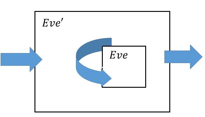
We show that the security of \(S'\) implies the security of \(S\) by transforming an adversary \(Eve\) breaking \(S\) into an adversary \(Eve'\) breaking \(S'\)
~ MathDefs ~
CS 127: Cryptography / Boaz Barak
Additional reading: Chapter 3 up to and including Section 3.3 in Katz Lindell book.
Recall our cast of characters- Alice and Bob want to communicate securely over a channel that is monitored by the nosy Eve. In the last lecture, we have seen the definition of perfect secrecy that guarantees that Eve cannot learn anything about their communication beyond what she already knew. However, this security came at a price. For every bit of communication, Alice and Bob have to exchange in advance a bit of a secret key. In fact, the proof of this result gives rise to the following simple Python program that can break every encryption scheme that uses, say, a \(128\) bit key, with a \(129\) bit message:
# Gets ciphertext as input and two potential plaintexts
# Positive return value means first is more likely,
# negative means second is more likely,
# 0 means both have same likelihood.
#
# We assume we have access to the function Decrypt(key,ciphertext)
def Distinguish(ciphertext,plaintext1,plaintext2):
    bias = 0
    key = [0,0,....,0] #128 0's
    while(sum(key)<128):
        p = Decrypt(key,ciphertext)
        if p==plaintext1: bias++
        if p==plaintext1: bias--
        increment(key)
    return bias

# increment key when thought of as a number sorted from least significant
# to most significant bit. Assume not all bits are 1.
def increment(key):
    i = key.index(0);
    for j in range(i-1): key[j]=0
    key[i]=1
Now, generating, distributing, and protecting huge keys causes immense logistical problems, which is why almost all encryption schemes used in practice do in fact utilize short keys (e.g., \(128\) bits long) with messages that can much longer (sometimes even terrabytes or more of data).
So, why can’t we use the above Python program to break all encryptions in the Internet and win infamy and fortune? We can in fact, but we’ll have to wait a really long time, since the loop in Distinguish will run \(2^{128}\) times, which will take much more than the lifetime of the universe to complete, even if we used all the computers on the planet.
However, the fact that this particular program is not a feasible attack, does not mean there does not exist a different attack. But this still suggests a tantalizing possibility: if we consider a relaxed version of perfect secrecy that restricts Eve to performing computations that can be done in this universe (e.g., less than \(2^{256}\) steps should be safe not just for human but for all potential alien civilizations) then can we bypass the impossibility result and allow the key to be much shorter than the message?
This in fact does seem to be the case, but as we’ve seen, defining security is a subtle task, and will take some care. As before, the way we avoid (at least some of) the pitfalls of so many cryptosystems in history is that we insist on very precisely defining what it means for a scheme to be secure.
Let us defer the discussion how one defines a function being computable in “less than \(T\) operations” and just say that there is a way to formally do so. Given the perfect secrecy definition we saw last time, a natural attempt for defining computational security would be the following:
Security Definition (First Attempt): An encryption scheme \((E,D)\) has \(t\) bits of computational security if for every two distinct plaintexts \(\{m_0,m_1\} \subseteq {\{0,1\}}^\ell\) and every strategy of Eve using at most \(2^t\) computational steps, if we choose at random \(b\in{\{0,1\}}\) and a random key \(k\in{\{0,1\}}^n\), then the probability that Eve guesses \(m_b\) after seeing \(E_k(m_b)\) is at most \(1/2\).
This seems a natural definition, but is in fact impossible to achieve if the key is shorter than the message. The reason is that if the message is even one bit longer we can always have a very efficient procedure (one that runs in time \(2^t\) for a very small \(t\)) that achieves success probability of about \(1/2 + 2^{-n-1}\) by guessing the key. (I.e., replace the loop in Distinguish by choosing the key at random.)
However, such tiny advantage does not seem very useful, and hence our actual definition will be the following:
Security Definition (Computational Security): An encryption scheme \((E,D)\) has \(t\) bits of computational security1 if for every two distinct plaintexts \(\{m_0,m_1\} \subseteq {\{0,1\}}^\ell\) and every strategy of Eve using at most \(2^t\) computatoinal steps, if we choose at random \(b\in{\{0,1\}}\) and a random key \(k\in{\{0,1\}}^n\), then the probability that Eve guesses \(m_b\) after seeing \(E_k(m_b)\) is at most \(1/2+2^{-t}\).
Having learned our lesson, let’s try to see that this strategy does give us the kind of conditions we desired. In particular, let’s verify that this definition implies the analogous condition to perfect secrecy.
Theorem: If \((E,D)\) is has \(t\) bits of computational/ security then every subset \(M \subseteq {\{0,1\}}^\ell\) and every strategy of Eve using at most \(2^t-(100\ell+100)\) computational steps, if we choose at random \(m\in M\) and a random key \(k\in{\{0,1\}}^n\), then the probability that Eve guesses \(m\) after seeing \(E_k(m_b)\) is at most \(1/|M|+2^{-t+1}\).
Before proving this theorem note that it gives us a pretty strong guarantee. In the exercises we will strengthen it even further showing that no matter what prior information Eve had on the message before, she will never get any non-negligible new information on it. One way to phrase it is that if your attacker used a \(256\)-bit secure encryption to encrypt a message, then your chances of getting to learn any additional information about it before the universe collapses are more or less the same as the chances that a fairy will materialize and whisper it in your ear.
Proof: The proof is rather similar to the equivalence of guessing one of two messages vs. one of many messages for perfect secrecy. However, in the computational context we need to be careful keeping track of Eve’s running time. In that proof we showed that if there exists:
and
An adversary \(Eve:{\{0,1\}}^o\rightarrow{\{0,1\}}^\ell\) such that
\[ \Pr_{m{\leftarrow_{\tiny R}}M, k{\leftarrow_{\tiny R}}{\{0,1\}}^n}[ Eve(E_k(m))=m ] > 1/|M| \]
Then there exist two messages \(m_0,m_1\) and an adversary \(Eve':{\{0,1\}}^0\rightarrow{\{0,1\}}^\ell\) such that \(\Pr_{b{\leftarrow_{\tiny R}}{\{0,1\}},k{\leftarrow_{\tiny R}}{\{0,1\}}^n}[Eve'(E_k(m_b))=m_b ] > 1/2\).
To adapt this proof to the computational setting and complete the proof of the current theorem we need to:
Show that if the probability of \(Eve\) succeeding was \(\tfrac{1}{|M|} + \epsilon\) then the probability of \(Eve'\) succeeding is at least \(\tfrac{1}{2} + \epsilon/2\).
Show that if \(Eve\) can be computed in \(T\) operations, then \(Eve'\) can be computed in \(T + 100\ell + 100\) operations.
The first point can be shown by simply doing the same proof more carefully, keeping track how the advantage over \(\tfrac{1}{|M|}\) for \(Eve\) translates into an advantage over \(\tfrac{1}{2}\) for \(Eve'\). The second point is obtained by looking at the definition of \(Eve'\) from that proof. On input \(c\), \(Eve'\) computed \(m=Eve(c)\) (which costs \(T\) operations) and then checked if \(m=m_0\) (which costs, say, at most \(5\ell\) operations), and then output either \(1\) or a random bit (which is a constant, say at most \(100\) operations). QED
Note: The proof of this theorem is a model to how a great many of the results in this course will look like. Generally we will have many theorems of the form:
“If there is a scheme \(S'\) satisfying security definition \(X'\) then there is a scheme \(S\) satisfying security definition \(X\)”
In this case \(X'\) was “having \(t\) bits of security” (hardness of distinguishing between encryptions of two ciphertexts) and \(X\) was the more general notion of hardness of getting a non-trivial advantage over guessing for an encryption of a random \(m\in M\). Also here the scheme \(S\) was the same as \(S'\), but generally that need not always be the case. All of these proofs will have the same global structure— we will assume towards a contradiction, that there is an efficient adversay strategy \(Eve\) demonstrating that \(S\) violates \(X\), and build from \(Eve\) a strategy \(Eve'\) demonstrating that \(S'\) violates \(X\). This is such an important point that it deserves repeating:
The way you show that if \(S'\) is secure then \(S\) is secure is by giving a transformation from an adversary that breaks \(S\) into an adversary that breaks \(S'\)
For computational security, we will always want that \(Eve'\) will be efficient if \(Eve\) is, and that will usually be the case because \(Eve'\) will simply use \(Eve\) as a black box, which it will not invoke too many times, and addition will use some polynomial time preprocessing and postprocessing. The more challenging parts of such proofs are typically:
Coming up with the strategy \(Eve'\).
Analyzing the probability of success and in particular showing that if \(Eve\) had non-negligible advantage then so will \(Eve'\).
We show that the security of \(S'\) implies the security of \(S\) by transforming an adversary \(Eve\) breaking \(S\) into an adversary \(Eve'\) breaking \(S'\)
For practical security, often every bit of security matters. We want our keys to be as short as possible and our schemes to be as fast as possible while satisfying a particular level of security. However, for understanding the principles behind encryption, keeping track of those bits can be a distraction, and so just like we do for algorithms, we will use asymptotic analysis (also known as big Oh notation) to sweep many of those details under the carpet.
To a first approximation, there will be only two types of running times we will encounter in this course:
Polynomial running time of the form \(d\cdot n^c\) for some constants \(d,c>0\) (or \(poly(n)=n^{O(1)}\) for short) , which we will consider as efficient
Exponential running time of the form \(2^{d\cdot n^{\epsilon}}\) for some constants \(d,\epsilon >0\) (or \(2^{n^{\Omega(1)}}\) for short) which we will consider as infeasible.2
Another way to say it is that in this course, if a scheme has any security at all, it will have at least \(n^{1/3}\) bits of security where \(n\) is the length of the key.
These are not all the theoretically possible running times. One can have intermediate functions such as \(n^{\log n}\) though we will generally not encounter those. To make things clean (and to correspond to standard terminology), we will say that an algorithm \(A\) is efficient if it runs in time \(poly(n)\) when \(n\) is its input length (which will always be the same, up to polynomial factors, as the key length). If \(\mu(n)\) is some probability that depends on the input/key length parameter \(n\), then we say that \(\mu(n)\) is negligible if it’s smaller than every polynomial. That is, for every \(c,d\) there is some \(N\), such that if \(n>N\) then \(\mu(n) < 1/(cn)^d\). Note that for every non-constant polynomials \(p,q\), \(\mu(n)\) is negligible if and only if the function \(\mu'(n) = p(\mu(q(n)))\) is negligible.
Note: The above definitions could be confusing if you haven’t encountered asymptotic analysis before. Reading the beginning of Chapter 3 (pages 43-51) in the KL book can be extremely useful. As a rule of thumb, if every time you see the word “polynomial” you imagine the function \(n^{10}\) and every time you see the word “negligible” you imagine the function \(2^{-sqrt{n}}\) then you will get the right intuition. What you need to remember is that negligible is much smaller than any inverse polynomial, while polynomials are closed under multiplication, and so we have the “equations” \(negligible\times polynomial = negligible\) and \(polynomial \times polynomial = polynomial\). As mentioned, in practice people really want to get as close as possible to \(n\) bits of security with an \(n\) bit key, but we would be happy as long as the security grows with the key, so when we say a scheme is “secure” you can think of it having \(\sqrt{n}\) bits of security (though any function growing faster than \(\log n\) would be fine as well).
From now on, we will require all of our encryption schemes to be efficient which means that the encryption and decryption algorithms should run in polynomial time. Security will mean that any efficient adversary can make at most a negligible gain in the probability of guessing the message over its a priori probability. That is, we make the following definition:
Security Definition (Computational Security): An encryption scheme \((E,D)\) is computationally secure if for every two distinct plaintexts \(\{m_0,m_1\} \subseteq {\{0,1\}}^\ell\) and every efficient strategy of Eve, if we choose at random \(b\in{\{0,1\}}\) and a random key \(k\in{\{0,1\}}^n\), then the probability that Eve guesses \(m_b\) after seeing \(E_k(m_b)\) is at most \(1/2+\mu(n)\) for some negligible function \(\mu(\cdot)\).
One more detail that we’ve so far ignored is what does it mean exactly for a function to be computable using at most \(T\) operations. Fortunately, when we don’t really care about the difference between \(T\) and, say, \(T^2\), then essentially every reasonable definition gives the same answer. Formally, we can use the notions of Turing machines or Boolean circuits to define complexity. For concreteness, lets define that a function \(F:{\{0,1\}}^n\rightarrow{\{0,1\}}^m\) has complexity there exists a Boolean circuit (that uses the AND, OR and NOT gates) with at most \(T\) gates that computes \(F\). We will often also consider probabilistic functions in which case we allow the circuit a RAND gate that outputs a single random bits. For more on circuit complexity you can take a look at Chapter 6 of my computational complexity textbook with Arora (see also draft on the web ).
The fact that we only care about asymptotics means you don’t really need to think of gates, etc.. when arguing in cryptography. However, it is comforting to know that this notion has a precise mathematical formulation. See the appendix below for a more precise formulation of this and some discussion.
We are now ready to make our first conjecture:
The Cipher Conjecture:3 There exists a computationally scure encryption scheme \((E,D)\) (where \(E,D\) are efficient) with a key of size \(n\) for messages of size \(n+1\).
A conjecture is a well defined mathematical statement which (1) we believe is true but (2) don’t know yet how to prove. Proving the cipher conjecture will be a great achievement and would in particular settle the P vs NP question, which is arguably the fundamental question of computer science. That is, the following is known to be a theorem (feel free to ignore it if you don’t know the definition of P and NP, though if it piques your curiousity, you can find more about it by reading the first two chapters of my book with Arora):
Theorem: If \(P=NP\) then there does not exist a computationally secure encryption with efficient \(E\) and \(D\) and where the message is longer than the key.
Proof idea: If \(P=NP\) then whenever we have a loop that searches through some domain to find some string that satisfies a particular property (like the loop in the Distinguish subroutine above that searches over all keys) then this loop can be sped up exponentially .
While it is very widely believed that \(P\neq NP\), at the moment we do not know how to prove this, and so have to settle for accepting the cipher conjecture as essentially an axiom, though we will see later in this course that we can show it follows from some seemingly weaker conjectures.
There are several reasons to believe the cipher conjecture. We now briefly mention some of them:
Intuition: If the cipher conjecture is false then it means that for every possible cipher we can make the exponential time attack described above become efficient. It seems “too good to be true” in a similar way that the assumption that P=NP seems too good to be true.
Concrete candidates: As we will see in the next lecture, there are several concrete candidate ciphers using keys shorter than messages for which despite tons of effort, no one knows how to break them. Some of them are widely used and hence governments and other benign or not so benign organizations have every reason to invest huge resources in trying to break them. Despite that as far as we know (and we know a little more after Snowden) there is no significant break known for the most popular ciphers. Moreover, there are other ciphers that can be based on canonical mathematical problems such as factoring large integers or decoding random linear codes that are immensely interesting in their own right independently of their cryptographic applications.
Minimalism: Clearly if the cipher conjecture is false then we also don’t have a secure encryption with a key, say, twice as long as the message. But it turns out the cipher conjecture is in fact necessary for essentially every cryptographic primitive, including not just private key and public key encryptions but also digital signatures, hash functions, pseudorandom generators, and more. That is, if the cipher conjecture is false then to a large extent crytpgoraphy does not exist, and so we essentially have to assume it if we want to do any kind of cryptography.
“Give me a place to stand, and I shall move the world” Archimedes, circa 250 BC
Every perfectly secure encryption scheme is clearly also computationally secure, and so if required a message of size \(n\) instead \(n+1\) then the conjecture would have been trivially satisfied by the one-time pad. However, having a message longer than the key by just a single bit does not seem that impressive. Sure, if we used such a scheme with \(128\)-bit long keys, our communication will be smaller by a factor of \(128/129\) (or a saving of about \(0.8\%\)) over the one-time pad, but this doesn’t seem worth the risk of using an unproven conjecture. However, it turns out that if we assume this rather weak condition, we can actually get a computationally secure encryption scheme with a message of size \(p(n)\) for every polynomial \(p(\cdot)\). In essence, we can fix a single \(n\)-bit long key and communicate securely as many bits as we want!
Moreover, this is just the beginning. There is a huge range of other useful cryptographic tools that we can obtain from this seemingly innocent conjecture: (We will see what all these names and some of these reductions mean later in the course.)
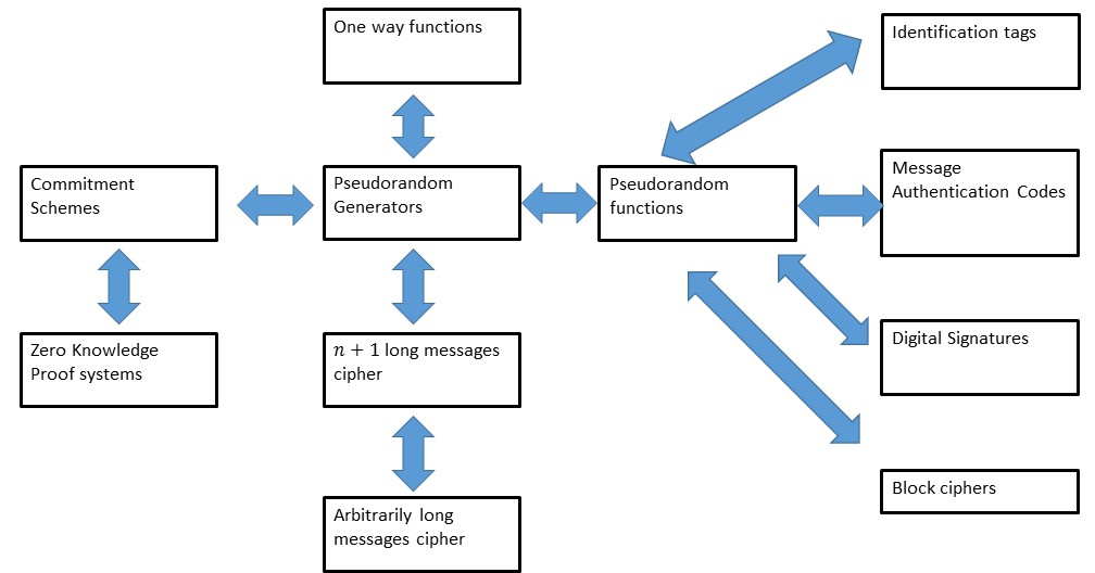
Web of reductions between notions equivalent to ciphers with larger than key messages
We will soon see the first of the many reductions we’ll learn in this course. Together this “web of reductions” forms the scientific core of cryptography, connecting many of the core concepts and enabling us to construct increasingly sophisticated tools based on relatively simple “axioms” such as the cipher conjecture.
The task of Eve in breaking an encryption scheme is to distinguish between an encryption of \(m_0\) and an encryption of \(m_1\). It turns out to be useful to consider this question of when two distributions are computationally indistinguishable more broadly:
Definition (Computational Indistinguishability): Let \(X\) and \(Y\) be two distributions over \({\{0,1\}}^o\). We say that \(X\) and \(Y\) are \((T,\epsilon)\)-computationally indistinguishable, denoted by \(X \approx_{T,\epsilon} Y\), if for every function \(Eve\) computable with at most \(T\) operations,
\[ | \Pr[ Eve(X) = 1 ] - \Pr[ Eve(Y) = 1 ] | \leq \epsilon \;. \]
We say that \(X\) and \(Y\) are simply computationally indistinguishable, denoted by \(X\approx Y\), if they are \((T,\epsilon)\) indistinguishable for every polynomial \(T(o)\) and inverse polynomial \(\epsilon(o)\).4
Note: The expression \(\Pr[ Eve(X)=1]\) can also be written as \({\mathbb{E}}[Eve(X)]\) (since we can assume that whenever \(Eve(x)\) does not output \(1\) it outputs zero). This notation will be useful for us sometimes.
We can use computational indistinguishability to phrase the definition of computational security more succinctly:
Theorem (C.I. phrasing of computational security): Let \((E,D)\) be a valid encryption scheme. Then \((E,D)\) is computationally secure if and only if for every two messages \(m_0,m_1 \in \{0,1\}^\ell\),
\[ \{ E_k(m_0) \} \approx \{ E_k(m_1) \} \]
where each of these two distributions is obtained by sampling a random \(k{\leftarrow_{\tiny R}}{\{0,1\}}^n\).
The proof is left as an Exercise in Homework 1.
One intuition for computational indistinguishability that it is related to some notion of distance. If two distributions are computationally indistinguishable, then we can think of them as “very close” to one another, at least as far as efficient observers are concerned. Intuitively, if \(X\) is close to \(Y\) and \(Y\) is close to \(Z\) then \(X\) should be close to \(Z\). Similarly if four distributions \(X,X',Y,Y'\) satisfy that \(X\) is close to \(Y\) and \(X'\) is close to \(Y'\), then you might expect that the distribution \((X,X')\) where we take two independent samples from \(X\) and \(X'\) respectively, is close to the distribution \((Y,Y')\) where we take two independent samples from \(Y\) and \(Y'\) respectively. We will now verify that these intuitions are in fact correct:
Lemma (Triangle Inequality for Computational Indistinguishability):5 Suppose \(\{ X_1 \} \approx_{T,\epsilon} \{ X_2 \} \approx_{T,\epsilon} \cdots \approx_{T,\epsilon} \{ X_m \}\). Then \(\{ X_1 \} \approx_{T, (m-1)\epsilon} \{ X_m \}\), where \(o\) is the length of the \(X_i\)’s.
Proof: Suppose that there exists a \(T\) time \(Eve\) such that
\[ |\Pr[ Eve(X_1)=1] - \Pr[ Eve(X_m)=1]| > (m-1)\epsilon \;. \]
Write
\[ \Pr[ Eve(X_1)=1] - \Pr[ Eve(X_m)=1] = \sum_{i=1}^{m-1} \left( \Pr[ Eve(X_i)=1] - \Pr[ Eve(X_{i+1})=1] \right) \;. \]
Thus,
\[ \sum_{i=1}^{m-1} \left| \Pr[ Eve(X_i)=1] - \Pr[ Eve(X_{i+1})=1] \right| > (m-1)\epsilon \]
and hence in particular there must exists some \(i\in\{1,\ldots,m-1\}\) such that
\[ \left| \Pr[ Eve(X_i)=1] - \Pr[ Eve(X_{i+1})=1] \right| > \epsilon \]
contradicting the assumption that \(\{ X_i \} \approx_{T,\epsilon} \{ X_{i+1} \}\) for all \(i\in\{1,\ldots,m-1\}\). QED
Lemma (Computational Indistinguishability is preserved under repetition): Suppose that \(X_1,\ldots,X_\ell,Y_1,\ldots,Y_\ell\) are distributions over \({\{0,1\}}^n\) such that \(X_i \approx_{T,\epsilon} Y_i\). Then \((X_1,\ldots,X_\ell) \approx_{T-10\ell n,\ell\epsilon} (Y_1,\ldots,Y_\ell)\).
Proof: For every \(i\in\{0,\ldots,\ell\}\) we define \(H_i\) to be the distribution \((X_1,\ldots,X_i,Y_{i+1},\ldots,Y_\ell)\). Clearly \(H_0 = (X_1,\ldots,X_\ell)\) and \(H_\ell = (Y_1,\ldots,Y_\ell)\). We will prove that for every \(i\), \(H_i \approx_{T-10\ell n,\epsilon} H_{i+1}\), and the proof will then follow from the triangle inequality (can you see why?). Indeed, suppose towards the sake of contradction that there was some \(i\in \{0,\ldots,\ell\}\) and some \(T-10\ell n\)-time \(Eve's:{\{0,1\}}^{n\ell}\rightarrow{\{0,1\}}\) such that
\[ \left| {\mathbb{E}}[ Eve'(H_i) ] - {\mathbb{E}}[ Eve(H_{i+1}) ] \right| > \epsilon\;. \]
In other words
\[ \left| {\mathbb{E}}_{X_1,\ldots,X_{i-1},Y_i,\ldots,Y_ell}[ Eve'(X_1,\ldots,X_{i-1},Y_i,\ldots,Y_\ell) ] - {\mathbb{E}}_{X_1,\ldots,X_i,Y_{i+1},\ldots,Y_ell}[ Eve'(X_1,\ldots,X_i,Y_{i+1},\ldots,Y_\ell) ] \right| > \epsilon\;. \]
By linearity of expectation we can write the difference of these two expectations as
\[ {\mathbb{E}}_{X_1,\ldots,X_{i-1},X_i,Y_i,Y_{i+1},\ldots,Y_ell}\left[ Eve'(X_1,\ldots,X_{i-1},Y_i,Y_{i+1},\ldots,Y_\ell) - Eve'(X_1,\ldots,X_{i-1},X_i,Y_{i+1},\ldots,Y_\ell) \right] \]
. By the averging principle6 this means that there exist some values \(x_1,\ldots,x_{i-1},y_{i+1},\ldots,y_\ell\) such that
\[ \left|{\mathbb{E}}_{X_i,Y_i}\left[ Eve'(x_1,\ldots,x_{i-1},Y_i,y_{i+1},\ldots,y_\ell) - Eve'(x_1,\ldots,x_{i-1},X_i,y_{i+1},\ldots,y_\ell) \right]\right|>\epsilon \]
Now \(X_i\) and \(Y_i\) are simply independent draws from the distributions \(X\) and \(Y\) respectively, and so if we define \(Eve(z) = Eve'(x_1,\ldots,x_{i-1},z,y_{i+1},\ldots,y_\ell)\) then \(Eve\) runs in time at most the running time of \(Eve\) plus \(2\ell n\) and it satisfies
\[ \left| {\mathbb{E}}_{X_i} [ Eve(X_i) ] - {\mathbb{E}}_{Y_i} [ Eve(Y_i) ] \right| > \epsilon \]
contradicting the assumption that \(X_i \approx_{T,\epsilon} Y_i\). QED
Note: The above proof illustrates a powerful technique known as the hybrid argument whereby we show that two distribution \(C^0\) and \(C^1\) are close to each other by coming up with a sequence of distributions \(H_0,\ldots,H_t\) such that \(H_t = C^1, H_0 = C^0\), and we can argue that \(H_i\) is close to \(H_{i+1}\) for all \(i\). This type of argument repeats itself time and again in cryptography, and so it is important to get comfortable with it.
We now turn to showing the length extension theorem. For a warm-up, let’s show that we can actually repeat encryptions to get an \(n/(n+1)\) saving.
Theorem (security of repetition): Suppose that \((E',D')\) is a computationally secure encryption scheme with \(n\) bit keys and \(n+1\) bit messages. Then the scheme \((E,D)\) where \(E_{k_1,\ldots,k_t}(m_1,\ldots,m_t)= (E'_{k_1}(m_1),\ldots, E'_{k_T}(m_t))\) and \(D_{k_1,\ldots,k_t}(c_1,\ldots,c_t)= (D'_{k_1}(c_1),\ldots, D'_{k_t}(c_t))\) is a computationally secure scheme with \(tn\) bit keys and \(t(n+1)\) bit messages.
Proof: This might seem “obvious” but in cryptography, even obvious facts are sometimes wrong, so it’s important to prove this formally. Luckily, this is a fairly straightforward implication of the fact that computational indisinguishability is preserved under many samples. That is, by the security of \((E',D')\) we know that for every two messages \(m,m' \in {\{0,1\}}^{n+1}\), \(E_k(m) \approx E_k(m')\) where \(k\) is chosen from the distribution \(U_n\). Therefore by the indistinguishability of many samples lemma, for every two tuples \(m_1,\ldots,m_t \in {\{0,1\}}^{n+1}\) and \(m'_1,\ldots,m'_t\in {\{0,1\}}^{n+1}\),
\[ (E'_{k_1}(m_1),\ldots,E'_{k_t}(m_t)) \approx (E'_{k_1}(m'_1),\ldots,E'_{k_t}(m'_t)) \]
for random \(k_1,\ldots,k_t\) chosen independently from \(U_n\) which is exactly the condition that \((E,D)\) is computationally secure. QED
Theorem (Length Extension of ciphers): Suppose that there exists a computaitonally secure encryption scheme \((E',D')\) with key length \(n\) and message length \(n+1\). Then for every polynomial \(t(n)\) there exists a computationally secure encryption scheme \((E,D)\) with key length \(n\) and message length \(t(n)\).
Proof: Let \(t=t(n)\). We are given a cipher \(E'\) which can encrypt \(n+1\)-bit long messages with an \(n\)-bit long key and we need to encrypt a \(t\)-bit long message \(m=(m_1,\ldots,m_t) \in {\{0,1\}}^t\). Our idea is simple (at least in hindsight). Let \(k_0 {\leftarrow_{\tiny R}}{\{0,1\}}^n\) be our key (which is chosen at random). To encrypt \(m\) using \(k_0\), the encryption function will choose \(t\) random strings \(k_1,\ldots, k_t {\leftarrow_{\tiny R}}{\{0,1\}}^n\).7 We will then encrypt the \(n+1\)-bit long message \((k_1,m_1)\) with the key \(k_0\) to obtain the ciphertext \(c_1\), then encrypt the \(n+1\)-bit long message \((k_2,m_2)\) with the key \(k_1\) to obtain the ciphertext \(c_2\), and so on and so forth until we encrypt the message \((k_t,m_t)\) with the key \(k_{t-1}\). We output \((c_1,\ldots,c_t)\) as the final ciphertext.8
To decrypt \((c_1,\ldots,c_t)\) using the key \(k_0\), first decrypt \(c_1\) to learn \((k_1,m_1)\), then use \(k_1\) to decrypt \(c_2\) to learn \((k_2,m_2)\), and so on until we use \(k_{t-1}\) to decrypt \(c_t\) and learn \((k_t,m_t)\). Finally we can simply output \((m_1,\ldots,m_t)\).
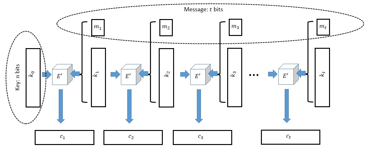
Constructing a cipher with \(t\) bit long messages from one with \(n+1\) long messages
The above are clearly valid encryption and decryption algorithms, and hence the real question becomes is it secure??. The intuition is that \(c_1\) hides all information about \((k_1,m_1)\) and so in particular the first bit of the message is encrypted securely, and \(k_1\) still can be treated as an unknown random string even to an adversary that saw \(c_1\). Thus, we can think of \(k_1\) as a random secret key for the encryption \(c_2\), and hence the second bit of the message is encrypted securely, and so on and so forth.
The above looks like a reasonable intuitive argument, but to make sure it’s true we need to give an actual proof. Let \(m,m' \in {\{0,1\}}^t\) be two messages. We need to show that \(E_{U_n}(m) \approx E_{U_n}(m')\). The heart of the proof will be the following claim:
Claim: Let \(\hat{E}\) be the algorithm that on input a message \(m\) and key \(k_0\) works like \(E\) except that its the \(i^{th}\) block contains \(E'_{k_{i-1}}(k'_i,m_i)\) where \(k'_i\) is a random string in \({\{0,1\}}^n\), that is chosen independently of everything else including the key \(k_i\). Then, for every message \(m\in{\{0,1\}}^t\)
\[ E_{U_n}(m) \approx \hat{E}_{U_n}(m) \;. \]
Note that \(\hat{E}\) is not a valid encryption scheme since it’s not at all clear there is a decryption algorithm for it. It is just an hypothetical tool we use for the proof. Once we prove the claim then we are done since we know that for every pair of message \(m,m'\), \(E_{U_n}(m) \approx \hat{E}_{U_n}(m)\) and \(E_{U_n}(m') \approx \hat{E}_{U_n}(m')\) but \(\hat{E}_{U_n}(m) \approx \hat{E}_{U_n}(m')\) since \(\hat{E}\) is essentially the same as the \(t\)-times repetition scheme we analyzed above. Thus by the triangle inequality we can conclude that \(E_{U_n}(m) \approx E_{U_n}(m')\) as we desired.
Proof of claim: We prove the claim by the hybrid method. For \(j\in \{0,\ldots, \ell\}\), let \(H_j\) be the distribution of ciphertexts where in the first \(j\) blocks we act like \(\hat{E}\) and in the last \(t-j\) blocks we act like \(E\). That is, we choose \(k_0,\ldots,k_t,k'_1,\ldots,k'_t\) independently at random from \(U_n\) and the \(i^{th}\) block of \(H_j\) is equal to \(E'_{k_{i-1}}(k_i,m_i)\) if \(i>j\) and is equal to \(E'_{k_{i-1}}(k'_i,m_i)\) if \(i\leq j\). Clearly, \(H_t = \hat{E}_{U_n}(m)\) and \(H_0 = E_{U_n}(m)\) and so it suffices to prove that for every \(j\), \(H_j \approx H_{j+1}\). Indeed, let \(j \in \{0,\ldots,\ell\}\) and suppose towards the sake of contradiction that there exists an efficient \(Eve'\) such that
\[ \left| {\mathbb{E}}[ Eve'(H_j)] - {\mathbb{E}}[ Eve'(H_{j+1})]\right|\geq \epsilon \;\;(*) \]
where \(\epsilon = \epsilon(n)\) is noticeable. By the averaging principle, there exists some fixed choice for \(k'_1,\ldots,k'_t,k_0,\ldots,k_{j-2},k_j,\ldots,k_t\) such that \((*)\) still holds. Note that in this case the only randomness is the choice of \(k_{j-1}{\leftarrow_{\tiny R}}U_n\) and moreover the first \(j-1\) blocks and the last \(t-j\) blocks of \(H_j\) and \(H_{j+1}\) would be identical and we can denote them by \(\alpha\) and \(\beta\) respectively and hence write \((*)\) as
\[ \left| {\mathbb{E}}_{k_{j-1}}[ Eve'(\alpha,E_{k_{j-1}}(k_{j},m_j),\beta) - Eve'(\alpha,E_{k_{j-1}}(k'_j,m_j),\beta) \right| \geq \epsilon \;\;(**) \]
But now consider the adversary \(Eve\) that is defined as \(Eve(c) = Eve'(\alpha,c,\beta)\). Then \(Eve\) is also efficient and by \((**)\) it can distinguish between \(E'_{U_n}(k_j,m_j)\) and \(E'_{U_n}(k'_j,m_j)\) thus contradicting the security of \((E',D')\). QED
For concreteness sake let us give a precise definition of what it means for a function or probabilistic process \(f\) mapping \(\zo^n\) to \(\zo^m\) to be computable using \(T\) operations:
Defintion: A probabilistic straightline program consists of a sequence of lines, each one of them one of the following forms:
a = b NAND c where a is a variable identifier and b, c are either variables that have been assigned a value before, or the constants 0 or 1.a = RAND where a is a variable identifier.a = INPUT where a is a variable identifier.OUTPUT b where b is a variable that has been assigned a value before.Given a program \(\pi\), we say that its size is the number of lines it contains. If the program has \(n\) INPUT commands and \(m\) OUTPUT commands, we identify it with the probabilistic process that maps \(\zo^n\) to \(\zo^m\) in the natural way. (That is, the variables all correspond to a single bit in \(\zo\), every time INPUT is called we take a new bit from the input, and every time OUTPUT is called we output a new bit.)
If \(F\) is a (probabilistic or deterministic) map of \(\zo^n\) to \(\zo^m\), the complexity of \(F\) is the size of the smallest program \(\pi\) that computes it.
If you haven’t taken a class such as CS121 before, you might wonder how such a simple model captures complicated programs that use loops, conditionals, and more complex data types than simply a bit in \(\zo\), not to mention some special purpose crypto-breaking devices that might involve tailor-made hardware. It turns out that it does (for the same reason we can compile complicated programming languages to run on silicon chips with a very limited instruction set). In fact, as far as we know, this model can capture even computations that happen in nature, whether it’s in a bee colony or the human brain (which contains about \(10^{10}\) neurons, so should in principle be simulatable by a program that has up to a few order of magnitudes the same number of lines). Crucially, for cryptography, we care about such programs not because we want to actually run them, but because we want to argue about their non existence.9 If we have a process that cannot be computed by a straightline program of length shorter than \(2^{128}>10^{38}\) then it seems safe to say that a computer the size of the human brain (or even all the human and nonhuman brains on this planet) will not be able to perform it either.
Advanced note: The computational model we use in this class is non uniform (corresponding to Boolean circuits) as opposed to uniform (corresponding to Turing machines). If this distinction doesn’t mean anything to you, you can ignore it as it won’t play a significant role in what we do next. It basically means that we do allow our programs to have hardwired constants of \(poly(n)\) bits where \(n\) is the input/key length.
This is a slight simplification of the typical notion of “\(t\) bits of security”. In the more standard definition we’d say that a scheme has \(t\) bits of security if for every \(t_1+t_2 \leq t\), an attacker running in \(2^{t_1}\) time can’t get success probability advantage more than \(2^{-t_2}\). However these two definitions only differ from one another by at most a factor of two. This may be important for practical applications (where the difference between \(64\) and \(32\) bits of security could be crucial) but won’t matter for our concerns.↩
Some texts reserve the term exponential to running times of the form \(2^{\epsilon n}\) for some \(\epsilon > 0\) and call running time of , say, \(2^{\sqrt{n}}\) subexponential . However, we will generally not make this distinction in this course.↩
As will be the case for other conjectures we talk about, the name “The Cipher Conjecture” is not a standard name, but rather one we’ll use in this course. In the literature this conjecture is mostly referred to as the conjecture of existence of one way functions, a notion we will learn about later. These two conjectures a priori seem quite different but have been shown to be equivalent.↩
This definition implicitly assumes that \(X\) and \(Y\) are actually parameterized by some number \(n\) (that is polynomially related to \(o\)) so for every polynomial \(T(o)\) and inverse polynomial \(\epsilon(o)\) we can take \(n\) to be large enough so that \(X\) and \(Y\) will be \((T,\epsilon)\) indistinguishable. In all the cases we will consider, the choice of the parameter \(n\) (which is usually the length of the key) will be clear from the context.↩
Results of this form are known as “triangle inequalities” since they can be viewed as generalizations of the statement that for every three points on the plane \(x,y,z\), the distance from \(x\) to \(z\) is not larger than the distance from \(x\) to \(y\) plus the distance from \(y\) to \(z\). In other words, the edge \(\overline{x,z}\) of the triangle \((x,y,z)\) is not longer than the sum of the lengths of the other two edges \(\overline{x,y}\) and \(\overline{y,z}\).↩
This is the principle that if the average grade in an exam was at least \(\alpha\) then someone must have gotten at least \(\alpha\), or in other words that if a real-valued random variable \(Z\) satisfies \({\mathbb{E}}Z \geq \alpha\) then \(\Pr[Z\geq \alpha]>0\).↩
Note that this makes the encryption function probabilistic but it does not increase the size of the key; while we didn’t explicitly say that the encryption can be probabilistic before, allowing this is absolutely fine and in fact will be necessary for some future security requirements.↩
The astute reader might note that the key \(k_t\) is actually not used anywhere in the encryption nor decryption and hence we could encrypt \(n\) more bits of the message instead in this final round. We used the current description for the sake of symmetry and simplicity of exposition.↩
An interesting potential exception to this principle that every natural process should be simulatable by a straightline program of comparable complexity are processes where the quantum mechanical notions of interference and entanglement play a significant role. We will talk about this notion of quantum computing towards the end of the course, though note that much of what we say does not really change when we add quantum into the picture. We can still capture these processes by straightline programs (that now have somewhat more complex form), and so most of what we’ll do just carries over in the same way to the quantum realm as long as we are fine with conjecturing the strong form of the Cipher conjecture and similar ones, namely that these are infeasible to break even for quantum computers. (All current evidence points toward these strong forms being true as well.)↩